2. Intro to Convolutional Neural Networks (CNNs) in PyTorch

May 24, 2024

In this second practical work, we’ll be experimenting with Convolutional Neural Networks (CNNs).

As Usual, Get Setup

Locally

You should have Jupyter installed and the following dependencies. You can use pip or any other dependency manager:

pip install torch torchvision matplotlib scikit-learn

You can add more dependencies if you think it is relevant.

In The Cloud (Google Colab)

Simply click here to open a Colab notebook in your browser. You’ll need to sign-in with you Google account.

In the first cell, add the following to install the dependencies:

!pip install torch torchvision matplotlib scikit-learn

Same here, you can add more dependencies if you think it is relevant.

Let’s Get Started

Deep neural networks are powerful tools for tackling computer vision problems. They often outperform the simpler Multi-Layer Perceptrons (MLPs) that we’ve explored previously on image tasks. In this tutorial, we’ll dive into building Convolutional Neural Networks (CNNs or ConvNets).

By the end of this tutorial, you will know:

• How Convolutional Neural Networks work
• Why CNNs are better than MLPs for image-related tasks
• How to create a CNN using PyTorch
• How to improve a CNN on a real use case

Why CNNs?

Convolutional Neural Networks (CNNs) are especially useful for working with images. Why? Because they are designed to recognize patterns, like edges, textures, and shapes, which are the building blocks of images.

One of the key features of CNNs is their receptive field. Think of it as a small window that scans over different parts of an image. Instead of looking at the whole picture at once, the CNN looks at small sections, one at a time, focusing on specific details. This helps the network detect local patterns and understand the image piece by piece.

Imagine trying to identify a cat in a photo. An MLP might struggle because it doesn’t naturally focus on parts of the image, it’ll try to look at everything at once. But a CNN starts by recognizing the edges of the cat, then the shapes like ears and eyes, and finally pieces these together to identify the whole cat. This “piece-by-piece” approach is why CNNs are so good at vision tasks and often outperform MLPs in these areas.

In other words, CNNs have a built-in advantage: they are designed to tackle tasks where it’s helpful to look at parts of an image (or a signal in general) and then combine those parts to understand the whole picture. This gives them a head start when learning the best weights during training because they are naturally better at processing image data than MLPs which have to figure out everything from scratch. However, it works both ways, this bias towards convolution might not be the optimal solution for image tasks, and we’re always looking for better methods. Spoiler alert: Nowadays, we also use transformers and actually even MLPs made a comeback for image tasks!

A CNN/ConvNet’s Architecture

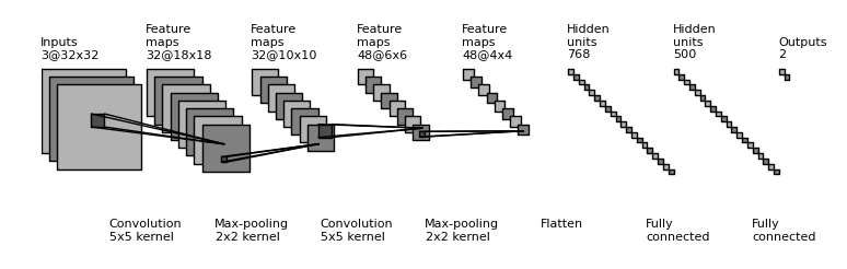
Let’s take a look at the image above. Starting on the right, you’ll see an Outputs layer with two outputs. This means the network makes two types of predictions, which could be for two different classes in a classification task or two separate regression outputs.

To the left of this, we have two layers with hidden units, known as Fully Connected or Linear layers. These are the same type of layers we know from a Multilayer Perceptron (MLP). So, even a Convolutional Neural Network (CNN) often includes MLP layers for making final predictions.

On the left side, we see Convolution layers followed by (Max) pooling layers.

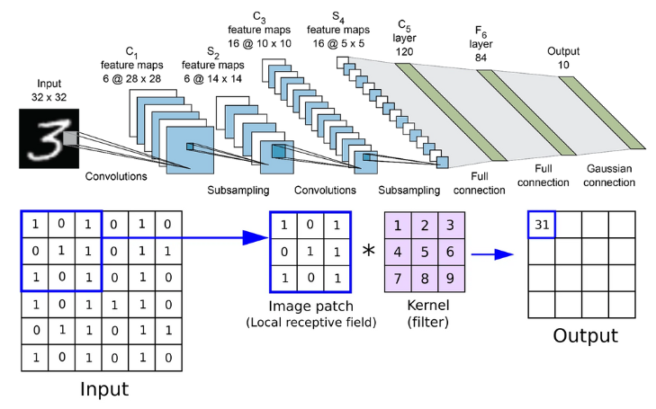
So, what is a convolution operation?

In simple terms, a convolution is a mathematical operation where one function modifies another. It’s like combining two sets of information to create a new set. This process helps the network focus on important features in the images, like edges and textures.

Here’s a more technical definition:

In mathematics (in particular, functional analysis), convolution is a mathematical operation on two functions ($f$ and $g$) that produces a third function ($f ∗ g$).

In our case, we will be mostly using 2D convolutions for images, but you can use 1D convolutions for other domains like text or audio data and even 3D convolutions for video data or MRI/CT scans.

In other words, a Convolutional layer takes two parts and creates a function that shows how one changes the other. Now that you’re getting familiar with neural networks, you know they have inputs that pass through layers with weights. From a Convolution perspective, these layers also have weights and they measure how much the inputs “trigger” or affect these weights.

By adjusting the weights during training, we teach the network to recognize specific patterns in the input data. For example, a Convolutional layer can learn to be triggered by certain features, like a nose, and connect this to the output class “human.”

Because CNNs use a sliding window (or kernel) that moves over the input data, they are translation invariant. This means they can detect features like a nose on a face regardless of where it appears in the image. This ability to recognize features anywhere in the image makes CNNs much more powerful for computer vision tasks than classic MLPs.

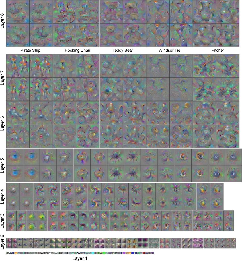
Exploring the Internals of CNNs

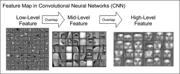
It can be interesting to understand what these models are learning internally to know why convolution with filters is an interesting architectural choice for a neural network. It definitely helps in understanding why they work.

Let’s take a look at what’s called an Activation Atlas below, specifically that of the InceptionV1 CNN classifier (also known as “GoogLeNet”) developed by Google that notably won the 2014 ImageNet Large Scale Visual Recognition Challenge.

Quick Dive into the Convolution Layer

As we already said above, the 2D convolution operation takes a filter (a fixed matrix of size $k×k$) and slides it across a signal (for example, an image). It is defined as follows:

$(f * g)(\mathbf{x}) = \int f(\mathbf{z}) g(\mathbf{x}-\mathbf{z}) d\mathbf{z}.$

However, the above definition is for continuous signals and we are working on a discrete signal (images contain pixels and there’s nothing inbetween). Let’s convert the above into a discrete formula:

$(f * g)(i, j) = \sum_a\sum_b f(a, b) g(i-a, j-b).$

You’ll note that there are two coordinates now, since we are working in two dimensions with image data.

Padding and Stride

To learn more about these and how to correctly compute your kernel size for a specific output, read this article which is quite well made.

Let’s build a CNN in PyTorch

To understand CNNs better, let’s take a look at an example first: Making a CNN recognize numbers!

Loading the Dataset

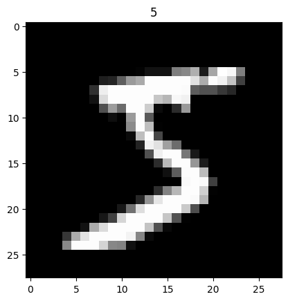
We’ll use the famous MNIST (Modified National Institute of Standards and Technology database) dataset, which is a collection of binarized handwritten digits.

Let’s first load the dataset using torchvision:

# Get the MNIST dataset
train_data = torchvision.datasets.MNIST(
    root='./mnist/',                                # Where to download the dataset
    train=True,                                     # Get the train data only
    transform=torchvision.transforms.ToTensor(),    # Convert a PIL Image or ndarray to tensor and scale the values accordingly
    download=True,                                  # Download the dataset only if you don't have it
)

Here’s what a digit looks like:

Now, the dataset contains 60k digits, so it’s going to be hard for us to train the model directly with the entire dataset in one batch because it might not fit in our GPU’s memory, so let’s train the model by making several passes of gradient descent by using mini-batches. We call this method mini-batch gradient descent:

# The number of images our DataLoader should return per batch
BATCH_SIZE = 64

# We create a DataLoader that will return mini-batches: the batch shape will be (batch_size=64, channels=1, width=28, height=28)
train_loader = DataLoader(dataset=train_data, batch_size=BATCH_SIZE, shuffle=True)

We will only use $64$ images per batch, and we use the shuffle option so the dataset is randomly shuffled which should give the model enough variety of numbers in one batch to learn a good model.

Designing the Model Architecture

Now, let’s design the model architecture:

class CNN(nn.Module):
    def __init__(self):
        super(CNN, self).__init__()
        self.conv1 = nn.Sequential(         # Input shape (1, 28, 28)
            nn.Conv2d(
                in_channels=1,              # Dnput depth/channels
                out_channels=16,            # Number of filters
                kernel_size=5,              # Filter size
                stride=1,                   # Filter movement/step
                padding=2,                  # If we want the same width and height of this image after conv2d, padding=(kernel_size-1)/2 if stride=1
            ),                              # Output shape (16, 28, 28)
            nn.ReLU(),                      # Activation
            nn.MaxPool2d(kernel_size=2),    # Choose max value in 2x2 area, output shape (16, 14, 14)
        )
        self.conv2 = nn.Sequential(         # Input shape (1, 28, 28)
            nn.Conv2d(16, 32, 5, 1, 2),     # Output shape (32, 14, 14)
            nn.ReLU(),                      # Activation
            nn.MaxPool2d(2),                # Output shape (32, 7, 7)
        )
        self.out = nn.Linear(32 * 7 * 7, 10)   # Linear layer, output 10 classes

    def forward(self, x):
        x = self.conv1(x)                   # Apply the first sequential block
        x = self.conv2(x)                   # Apply the second sequential block
        x = x.view(x.size(0), -1)           # Flatten the output of conv2d to (batch_size, 32 * 7 * 7)
        output = self.out(x)
        return output, x    # Return x for visualization

Let’s visualize the above model:

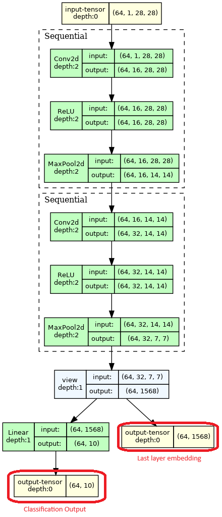
Let’s understand the flow and the architecture:

• 1 input: A batch ($bs=64$) of binarized $28*28$ images, meaning $1$ channel per image
• 2 Sequential blocks: Each block is composed of 3 operations
  • Conv2d: A 2d convolution operation that will create filters that will activate on features on the image and subsequent feature maps
  • ReLU: A non-linear activation function as usual
  • MaxPool2d: Max Pooling is an operation of dimensionality reduction. It basically reduces the feature map’s size by a factor $f$ by looking at blocks of size $f × f$ and taking the max value of each block. This has several benefits:
    • Compression: Looking at every little detail in the image/feature map forces the model to overfit by remembering too much information. This operation forces the network to work with reduced dimensions in the next layer so it has to focus on more global features to be able to store features with less parameters. Using less parameters in subsequent layers also helps the model use less compute power.
    • Helps the model focus on important features: By only taking the values that activated most, Max Pooling forces the model to focus on important features like edges, textures, etc, that truly distinguish an object from another.
    • Helps a bit with Transformation invariance: Since we’re focusing less on micro details, the model doesn’t need to look for very specific details when looking for a feature, it looks more for an approximation of this feature which helps if the feature has as slight transformation applied to it like translation, rotation, etc. However, it doesn’t help as much if the transformation is significant, only more data or data augmentation helps here with CNNs.
    • For more details, read more here.
• 1 reshape operation: This operation just rearranges the values in the tensor, but why is this needed? In our case we eventually want to output a 1D vector of size $10$ that will contain the classification results for each number class from $0$ to $9$. We thus need to go from our multiple dimension feature maps to an even more compressed representation using a linear layer. So this operations just rearranges the tensor from 3D to 1D, the values stay the same, but shapes go from $(batch\_size, filters, feature\_map\_x, feature\_map\_y)$ to $(batch\_size, filters×feature\_map\_x × feature\_map\_y)$
• 2 outputs: In practice your neural network can have several possible outputs with different purposes, also called heads. They can be used to perform several tasks with the same backbone (base of the model before the output that learns useful features that can be reused across tasks).
  • Classification output: This is classic, we just use a linear layer that will convert from the CNN’s representation to the $10$ digits classes classification.
  • Last layer embedding output: This output is only used a visualization/debug output, we basically get the last internal representation (embedding) inside of the network so we can plot it and understand how our model represents our data. We’ll see how to do that below.

Training the Model

Training this model is very similar to what we did in the previous practical work.

We first instantiate the model:

device = torch.device("cuda" if torch.cuda.is_available() else "cpu")

cnn = CNN().to(device)

Then we instantiate the optimizer (AdamW) and loss function (Cross Entropy). We’ll use a new optimizer this time just for the sake of showing you what are the best optimizers being used nowadays. AdamW is one of the optimizers which converges the fastest in most cases. It is a stochastic gradient descent method that is based on adaptive estimation of first-order (the mean) and second-order moments (the variance) with an added method to decay weights per the techniques discussed in the paper, ‘Decoupled Weight Decay Regularization’ by Loshchilov, Hutter et al., 2019.:

# The Learning Rate (LR)
LR = 0.001

optimizer = torch.optim.AdamW(cnn.parameters(), lr=LR)  # We optimize all the parameters of the CNN
loss_func = nn.CrossEntropyLoss()                       # The loss

The difference here is that we use a device variable so we can ask PyTorch to train on GPU if we have one, which makes training much faster. Now let’s train the model:

EPOCH = 1

for epoch in range(EPOCH):
    for step, (b_x, b_y) in enumerate(train_loader):   # gives batch data, normalize x when iterate train_loader
        b_x = b_x.to(device)  # Batch X: Image data that we move to our device
        b_y = b_y.to(device)  # Batch Y: Label data that we move to our device
        
        output = cnn(b_x)[0]            # CNN's classification output, this is the first head of the network
        
        loss = loss_func(output, b_y)   # The Cross-Entropy loss
        
        optimizer.zero_grad()           # We clear the gradients every training step
        loss.backward()                 # Backpropagation and compute gradients
        optimizer.step()                # Use the computed gradients to do gradient descent

Let’s Do Some Visualization

Let’s use the second head of our network to visualize the learned representation of the network using a method that projects high dimentional vectors to 2D. Why would we need this since we get back a 1D representation vector (embedding) for each image already? Well, this 1D vector contains $1568$ values, aka features, ideally we’d like to plot it in 2D and 2D means we need two coordinates (which are a type of feature) for each image relatively to eachother so we can actually visualize the network’s representation. This representation is only valid relatively to other images given as input to the network.

To get this representation we use dimensionality reduction methods that will go from $X$ features to $3$ or even $2$ features which we’ll use to plot them on a 2D plot. Many methods exist for this like Kernel PCA, UMAP or t-SNE. Here we use t-SNE (t-distributed stochastic neighbor embedding):

def plot_embeddings_with_labels(low_d_weights, labels, accuracy):
    plt.cla()
    # Get X and Y coordinates from each t-SNE projected embeddings
    X, Y = low_d_weights[:, 0], low_d_weights[:, 1]
    for x, y, s in zip(X, Y, labels):
        # Each number class will have its own color
        c = cm.rainbow(int(255 * s / 9))
        plt.text(x, y, s, backgroundcolor=c, fontsize=9)

    plt.xlim(X.min(), X.max())
    plt.ylim(Y.min(), Y.max())
    plt.title(f"Last layer embedding space. Accuracy={accuracy:.2f}")
    
    # Plot the embeddings
    plt.show()

def plot(cnn, test_x, test_y, loss, epoch, device):
    # Run the model on our test data
    test_output, last_layer = cnn(test_x.to(device))
    # Get the class with max value which is the predicted class by the model
    pred_y = torch.max(test_output, 1)[1].data.squeeze().detach().cpu()
    # Compute an accuracy metric
    accuracy = (pred_y == test_y).sum().item() / float(test_y.size(0))

    print(f"Epoch:{epoch} | train loss: {loss.data:.4f} | test accuracy: {accuracy:.2f}")

    # Visualization of trained flatten layer using T-SNE
    tsne = TSNE(perplexity=30, n_components=2, init='pca', n_iter=5000, random_state=42)

    # We'll only display a few of them otherwise the plot will be too crowded and hard to read
    plot_only = 500

    # Project embeddings to 2D using t-SNE 
    low_dim_embs = tsne.fit_transform(last_layer.detach().cpu().numpy()[:plot_only, :])
    labels = test_y.numpy()[:plot_only]
    plot_embeddings_with_labels(low_dim_embs, labels, accuracy)

Put this piece of code inside the training loop and run it only every few steps since it is compute intensive.

This is what this looks like every few steps:

Now that we understand the basics, let’s solve a more interesting task!

Let's Aim Bigger:

What is Super-Resolution?

Super resolution is the process of taking a low-resolution image and upscaling it to recover, or more accurately, extrapolate details at a higher resolution. The term “extrapolate” is used because the additional details do not actually exist in the original image. Unlike interpolation algorithms such as bicubic or Lanczos resampling, which do not require machine learning, super resolution uses advanced techniques to infer and generate these new details using neural networks.

Let’s not forget that even these “simpler” interpolation methods are quite good baselines that can be hard to beat, even production-ready methods such as AMD Radeon™ Super Resolution for video game super-resolution use Lanczos at their core. However, methods such as Nvidia DLSS use deep learning and offer better results and performance in general (shameless plug since I worked on DLSS v1 😃).

History

The general idea is that we have a low resolution (LR) image and we want to get to a high resolution (HR) image. One of the first papers to do so using deep learning in an end-to-end fashion was “Image Super-Resolution Using Deep Convolutional Networks, Chao Dong et al, 2014”.

To enhance a low-resolution image, the image is first upscaled to the desired super-resolution size using bicubic interpolation, resulting in an interpolated image $Y$. The aim is to recover an image $F(Y)$ from $Y$ that resembles the high-resolution image $X$ we want to obtain in terms of dimensions. Despite the $Y$ having the same dimensions as $X$, it is still referred to as low-resolution.

The process then involves three main operations:

1. Patch extraction and representation, where overlapping patches from $Y$ are extracted and represented as high-dimensional vectors to form feature maps.
2. Non-linear mapping, which transforms each high-dimensional vector into another high-dimensional vector representing high-resolution patches, forming a new set of feature maps.
3. Reconstruction, which combines these high-resolution patch representations to generate the final high-resolution image similar to $X$. These operations collectively form a convolutional neural network, as illustrated in the above figure.

Now, something that isn’t ideal with their approach is that they first upscale the image using bicubic interpolation to get the final shape they need to operate on. This really isn’t optimal at all since it introduces a bias from the bicubic interpolation!

Let’s Improve The Architecture

Let’s improve their architecture step-by-step by going for an architecture that takes the low resolution image directly as input.

A few things to notice here:

• The input dimensions of the network $(1, 1, H, W)$ are $(batch\_size, channels, height, width)$
• Why is $channels = 1$?
• What’s the PixelShuffle operation?
• Is padding needed in the convolutions? Read more about this here.

Let’s answer a few of these questions.

RGB for Images, right? Nah, Let’s Switch To YCbCr!

Computer displays are driven by red ($R$), green ($G$), and blue ($B$) voltage signals. These signals are efficient in describing how color physically works. However, these RGB signals are not efficient to store since they have a lot of redundancy and usually we want to have the best compromise between size and quality.

On top of that, and that’s very important for us here, the human vision works in a specific way which was can use to our advantage: Due to the densities of color and brightness-sensitive receptors in the human eye, humans can see considerably more fine detail in the brightness of an image (the $Y$ component) than in the hue and color saturation of an image (the $Cb$ and $Cr$ components). If you zoom in on the Cb and Cr componenets of the image below, you’ll see that the details are indeed there but our eyes have a much harder time at seeing them.

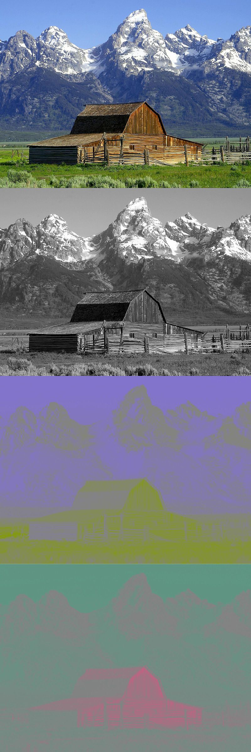
This property enables us to decorrelate “detail” from “color” information in YCbCr while RGB has luminance information spread out across $R$, $G$ and $B$. And as you know, the less correlation we have between features (or components in this case) in data, the more we can compress this data. JPEG actually uses YCbCr since it can help better compress the final image.

Now, why would we need this inside a neural network?

Because for our first simple super resolution network, which just adds more details to an image, we’ll only apply super-resolution on the “details” or $Y$ channel and it’ll be enough to recombine it with bicubic upscaled $Cb$ and $Cr$ channels which we’ll convert back to RGB so we can see the final image.

This basically explains why $channels = 1$ in our network, because we only keep the luminance/detail channel for our super-resolution needs.

What’s Pixel Shuffle?

If you look at our network architecture above, we want to get from an image input size of $(H, W)$ to an image output size of $(H × 2, W × 2)$ to achieve a super-resolution scaling of $2×$. To achieve this, there are several solutions that exist, of which are:

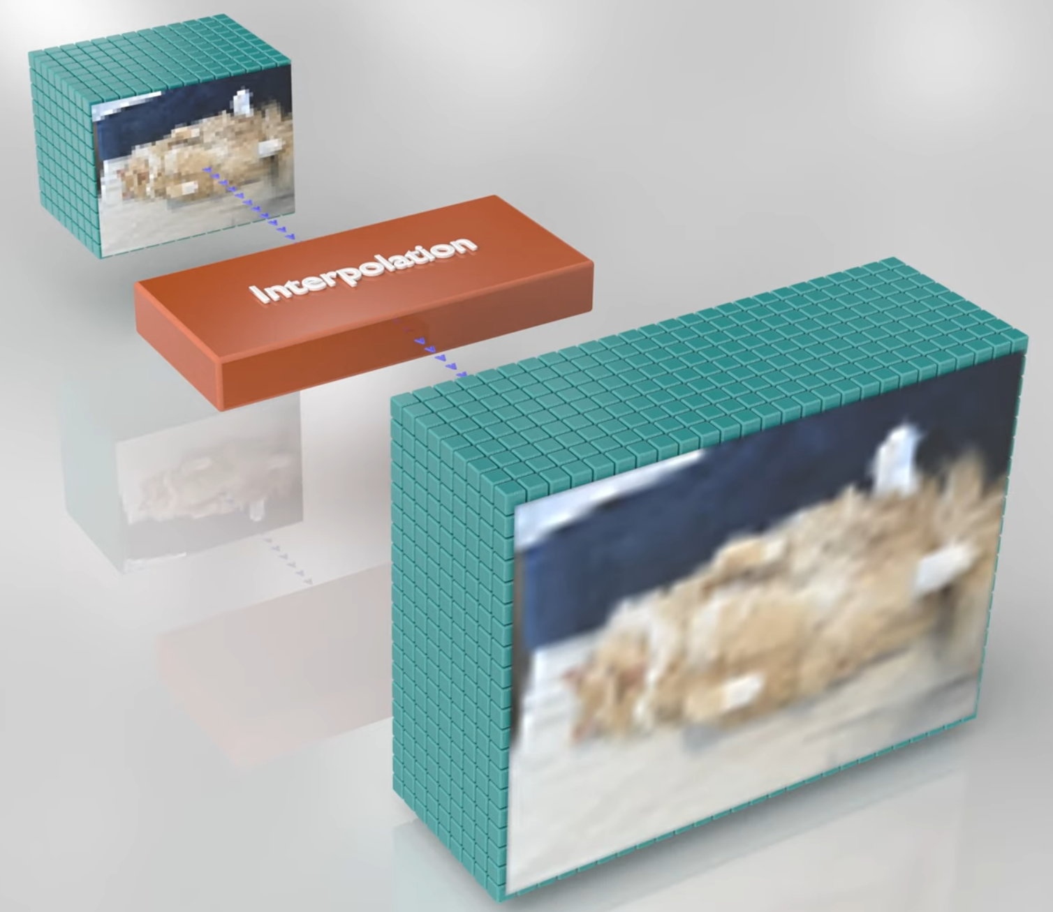
• Interpolation methods: This simply applies an interpolation algorithm such as bicubic interpolation and gives us the correct output size, but at the price of blurry features.
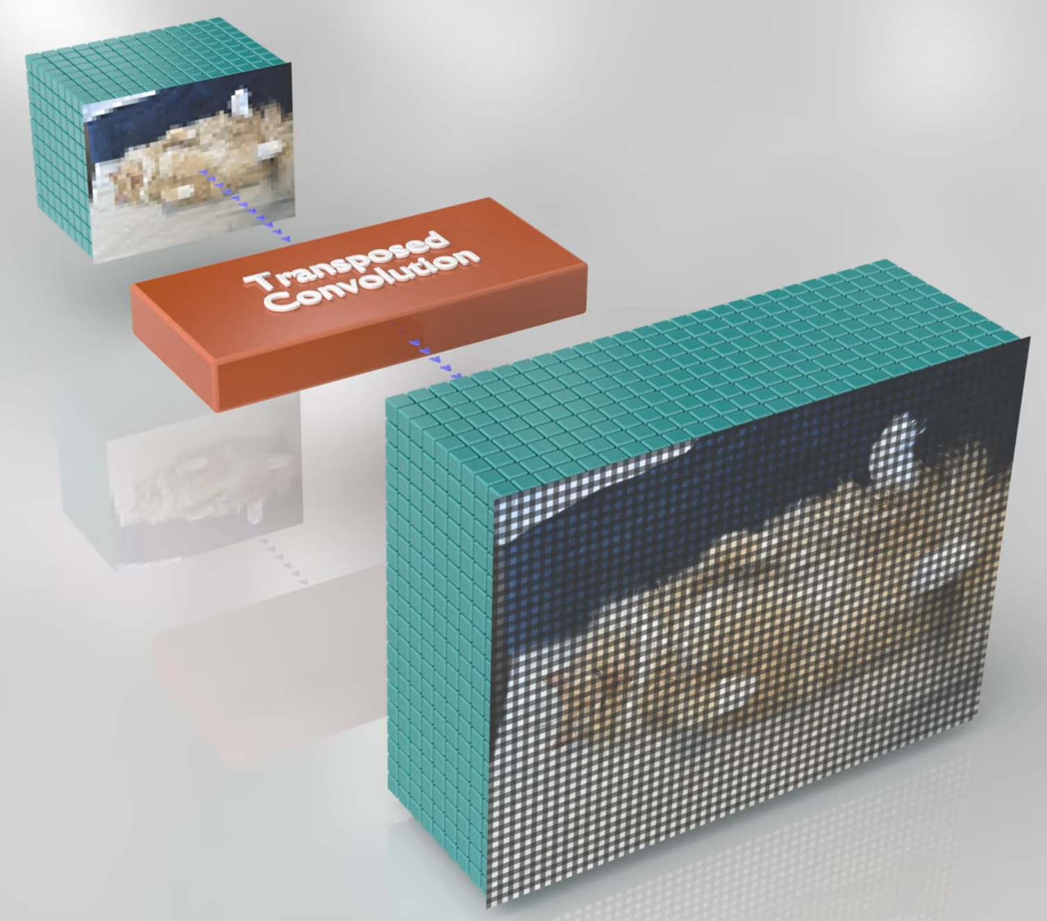
• Transposed convolution: This is a different type of convolution that outputs a bigger signal by effectively spacing the signal before applying convolution to it, so it makes it bigger in the output, but it’s also a form of interpolation in the end that discards part of the information. More details here.

Pixel Shuffle was introduced to circumvent all the above issues by rearranging the input tensors from depth to spatial features. This means that as we go deeper in our network, we’ll create enough convolution filters (this is the depth part) that will in the end create feature maps ordered by depth to be used to store the new details we will add to our image by rearranging them from depth to space.

This means that our network will do what any usual CNN does by stacking convolutional layers with a lot of filters to encode the input image into hidden feature maps and then we’ll reduce these filters until the end of the network until we have only enough left for storing the new image details.

So at the end of the network in our case, we’ll have a final convolution layer that will store enough filters to propagate them into the spatial dimensions of our model. Let’s trace the shape of the image feature maps through our network:

• Input luminance (in black & white) image size is $(1, 1, H, W)$
• Classic convolutional process with $ReLU(conv2d(X))$ operations
• At the end of convolutional layers, we downscale filters to exactly $(1, 4, H, W)$
  • Why? Because scaling an image $2×$ means scaling each of its dimensions (width and height) by $2×$, which is a $4×$ factor in the end
• Pixel Shuffle propagates the $4$ filters into $2×$ on the width and $2×$ on the height dimensions: $(1, 1, H × 2, W × 2)$

From this, we can conclude that the Pixel Shuffle formula works for any resolution upscaling factor: It just rearranges elements from a tensor of shape $(∗,C×r^2,H,W)$ to a tensor of shape $(∗,C,H×r,W×r)$, where $r$ is an upscale factor.

PyTorch fortunately defines Pixel Shuffle as a very simple layer for us that we can just plug into our network.

Train Your Model!

To get started with this task, you should go to the Practical Work 2 GitHub repository here. You’ll need to plug your model in the model.py file, the rest (data loading, training, testing and running the model) is done for you so you don’t have to think about it, but it’s very similar to what you’ve already seen before.

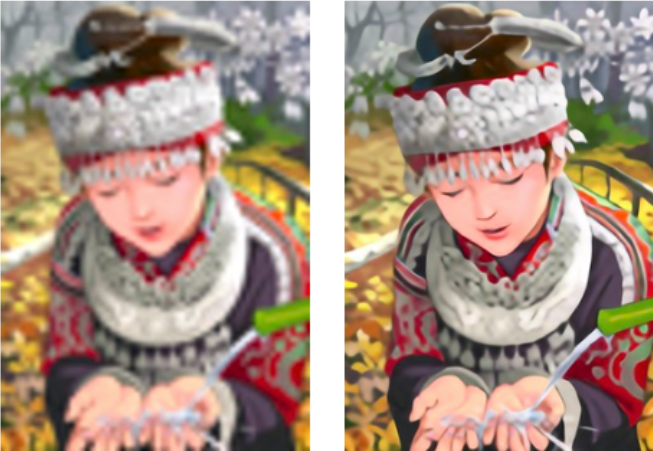
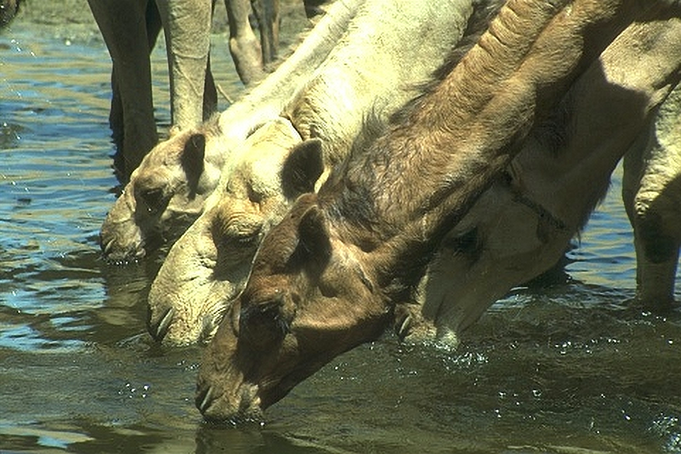
You should get a network that’ll create higher resolution images such as this after training:

Last Exercise: DIY Pixel Shuffle!

Read the documentation of einops here.

You’re Done!

Great job, you made it this far!

Class Students

Send it on the associated MS Teams Assignment.

Anyone else

Send it to my email adress with the subject Practical Work 2: chady1.dimachkie@epita.fr

Don’t hesitate if you have any questions!

→ Coming Next: Practical Work 3