3. Intro to Denoising Diffusion Probabilistic Models (DDPMs) for Image Generation

June 3, 2024

In this third practical work, we’ll be experimenting with Denoising Diffusion Probabilistic Models (DDPMs).

As Usual, Get Setup

Locally

You should have Jupyter installed and the following dependencies. You can use pip or any other dependency manager:

pip install torch einops datasets matplotlib tqdm

You can add more dependencies if you think it is relevant.

In The Cloud (Google Colab)

Simply click here to open a Colab notebook in your browser. You’ll need to sign-in with you Google account.

In the first cell, add the following to install the dependencies:

!pip install torch einops datasets matplotlib tqdm

Same here, you can add more dependencies if you think it is relevant.

Let’s Get Started

You’ve probably already heard of DALL-E, Midjourney or even Stable Diffusion where you give them a piece of text with instruction (prompt) and they generate any image you can ask for.

Denoising Diffusion Probabilistic Models (DDPMs) is a class of Diffusion Models. They work really well and they’ve beaten other long standing architectures like Generative Adversarial Networks (GANs) at image generation tasks.

In this practical work, we’ll be implementing only the image generation side without the text encoder part.

Denoising Diffusion Probabilistic Models (DDPMs)

In this section, we’ll be exploring the original “Denoising Diffusion Probabilistic Models” paper by Ho et al, 2020.

The Main Idea

These models have already existed for a while, but it took quite some iterations to make them work as well as today. It first started off from ideas from “non-equilibrium statistical physics” which sounds quite complex but is essentially the science of evolution of isolated systems over time according to deterministic equations. Examples of these systems include:

• Heat distribution inside of a material
• Electric currents carried by the motion of charges in a conductor
• Chemical Reactions

Ok, but what does this have to do with Machine Learning?

Well, this method was first introduced in the paper titled “Deep Unsupervised Learning using Nonequilibrium Thermodynamics” by Sohl-Dickstein et al, 2015. In their paper, they propose the following method:

The essential idea, inspired by non-equilibrium statistical physics, is to systematically and slowly destroy structure in a data distribution through an iterative forward diffusion process. We then learn a reverse diffusion process that restores structure in data, yielding a highly flexible and tractable generative model of the data.

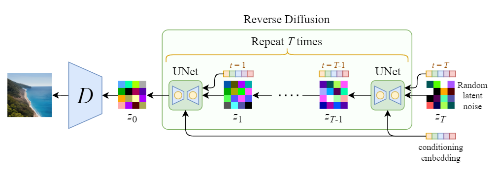
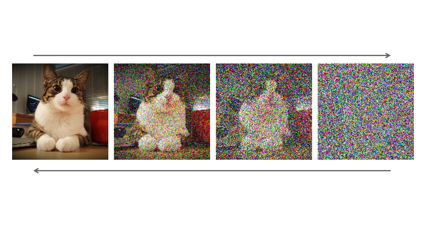
So basically, this approach uses a predefined step that gradually adds noise to an image until we get only pure noise. The method then learns to reverse this noise process to get back to the original image, so it is a denoising process. Ultimately, this method uses a pure noise image as a starting point and reverses the noise until we get an image that makes sense.

To explain further why this is related to “equilibrium statistical physics”: The noise we start with can be visualized as a field of particles that are completely disorganized (non-equilibrium) at the beginning but want to find the point where they are organized (equilibrium) and they can only follow the rules they have at their disposal to reach this equilibrium, which are the laws of physics in this case. It’s like waiting for a kettle of boiled water to cool down, where the water particles are already heated, so they bounce everywhere, the water just goes naturally to a more stable state of being still and cold by following the laws of thermodynamics.

In our case, the “non-equilibrium” is the noise image, the “laws of physics” will be the learned reverse diffusion process and the “equilibrium” state to which it will converge to an image that makes sense.

Let’s Get Into The Details

A (denoising) diffusion model isn’t that complex if you compare it to other generative models such as Normalizing Flows, Generative Adversarial Networks (GANs) or Variational AutoEncoders (VAEs): They all convert noise from some a simple distribution, such as Gaussian noise, to a data sample, such as an image. Basically, they’re all neural network methods that learn to gradually denoise data starting from pure noise.

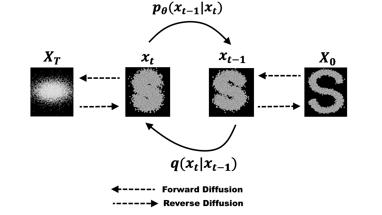
As we’ve said, there are 2 processes in diffusion models:

• Forward Diffusion: The predefined process $q$ of adding Gaussian noise to an image until we get only 100% (Gaussian) noise
• Reverse Diffusion: A learned process of denoising an image, where you start from a Gaussian noise and try to reverse (more like rearrange) the noise until you get an image

Both processes are time-based, so they happen in a predefined number of steps $T$, the paper uses $T = 1000$ which is actually a huge number nowadays where we can do under $10$ steps.

Forward Diffusion Process

At $t = 0$ you take an image $x_0$ from your train set and then apply to it Gaussian noise in an appropriate way (following a schedule which we’ll discuss later) at each time step $t$. By the end, $T = 1000$ or before if you’re lucky, you’ll end up with a noise image, this noise will actually have converged to what’s called an isotropic Gaussian distribution. This specific type of noise has properties that make it much simpler to manipulate in the equations that follow, as opposed to anisotropic distribution. Read more about this here if you’re interested.

Let’s describe the distribution of our training image dataset as $q(x_0)$ from which we can sample, basically get images from, this way: $x_0 \sim q(x_0)$

Let’s also define the Forward diffusion process at each time step $t$: $q(x_t|x_{t-1}) = \mathcal{N}(x_t; \sqrt{1 - \beta_t}x_{t-1},\beta_t \mathbf{I})$, where $\beta_1,…,\beta_T$ ($0 < \beta_t < 1$) is called the variance schedule because it’ll modulate the variance of the Gaussian distribution we are sampling from, making it bigger each time step (meaning there is one $\beta_t$ for each time step), meaning we’ll have more spread out noise as the time step $t$ increases.

$q(x_t|x_{t-1})$ just means, from the previous image we added noise to, with $x_0$ being the original image without noise, what is the next image with one noise step added to. $\mathcal{N}$ is a Normal distribution, also called a Gaussian distribution, which has two parameters: the mean $\mu$ and variance $\sigma^2 \geq 0$ (Read more here in case you forgot). A nice trick to get the complex Gaussian noise sample we need above from a simple standard normal distribution $\mathcal{N}(\mathbf{0}, \mathbf{I})$ with mean $\mu = 0$ and variance $\sigma = 1$ is to get a sample from this simpler Gaussian distribution and then center and scale it by doing this: $x_t = \sqrt{1 - \beta_t} x_{t-1} + \sqrt{\beta_t} \mathbf{\epsilon}$, where $\mathbf{\epsilon} \sim \mathcal{N}(\mathbf{0}, \mathbf{I})$.

This was for going from one time step to another. The entire process can be summarized as a Markov chain that gradually adds Gaussian noise to the data: $q(x_{1:T}|x_0) = \prod_{t=1}^{T} q(x_t|x_{t-1})$. This just means that each step depends on the previous one for the next result, like a chain.

$\beta$-Variance Schedule

As we said, the $\beta_t$ are different at each time step, but what values should we assign each?

The original DDPM paper uses a linear schedule, basically just a linear function that increases from $\beta_1 = 10^{-4}$ to $\beta_T = 0.02$.

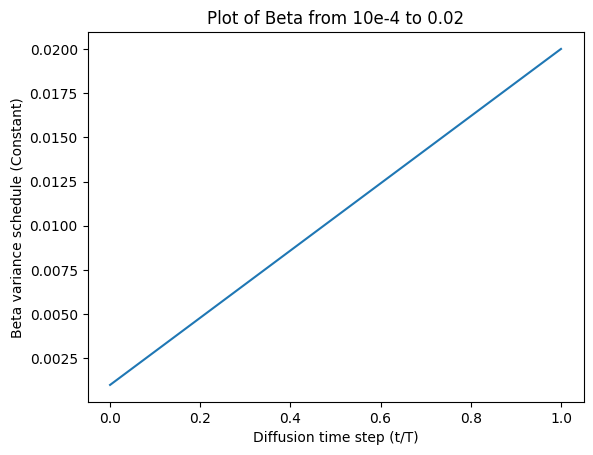
These constants were chosen to be small relative to data scaled to $[−1, 1]$, ensuring that reverse and forward processes have approximately the same functional form while keeping the signal-to-noise ratio at $x_T$ as small as possible.

Reverse Diffusion Process

Looking back again at the figure above, we see that we actually go back from noisy to less noisy in the reverse process. If we were able to find $p_{\theta(x_{t-1|t})}$, which knowing the noisier image at $x_{t-1}$ could get us a less noisy image $x_{t}$, it would be amazing (you’ll also notice that indices are reversed compared to $q(x_t|x_{t-1})$, since this is the reverse process). Unfortunately, it’s impossible to get a closed form formula that will give us the solution, so to solve that we’ll simply use a neural network to approximate this conditional probability distribution $p_{\theta(x_{t-1|t})}$ with $\theta$ being the parameters of the neural network, updated by usual gradient descent.

If we try to deconstruct the process of learning this probability distribution function to simplify things for us, we could assume that the reverse process is also Gaussian, similarly to the forward process. A Gaussian distribution has, again, a mean parameter $\mu$ and a variance $\Sigma$. Let’s write what this function would look like so far: $p_{\theta(x_{t-1|t})} = \mathcal{N}(x_{t-1}; \mu_\theta(x_{t},t), \Sigma_\theta (x_{t},t))$, where we add $\theta$ subscripts to each because we’ll want to learn them with our neural network parameters and they’ll take as input the current noisy image $x_t$ and the current time step $t$. This is amazing because we simplified the problem to just learning the mean and variance parameters of a Gaussian distribution, can’t get simpler right?

Actually it does!

The authors of the paper decided that they’ll keep the variance fixed and let the neural network learn only the mean $\mu_{\theta}$, so the variance above becomes: $\Sigma_\theta (x_{t},t) = \sigma^2_t \mathbf{I}$ and they set $\sigma^2 = \beta_t$, we come back to our $\beta_t$ constants from above!

What About the Loss Function?

This section is the complex part and will defer most of the details to different papers and articles for those who’d like to understand the details more in-depth.

According to the paper it’s all simple:

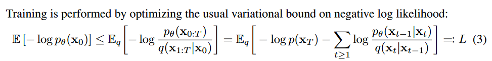
But what’s this “usual variational bound on negative log likelihood”? Basically, it’s an observation that the forward $q$ and reverse $p_{\theta}$ processes can be seen as a Variational Auto-Encoder (VAE) (first described in the paper “Auto-Encoding Variational Bayes”, Kingma et al., 2013 for more details). This formulation allows us to use the “Variational lower bound” which basically helps us approximate the log-likelihood of the train data using gradient-based methods by finding a lower bound to this log-likelihood. This tells us that $log(p_{\theta}(x_0)) > L$, where $L$ is the equation above from the paper. Meaning that if we maximize the negative of it $-log(p_{\theta}(x_0))$ through optimization then we’ll find a solution to our problem. Why maximizing? Because it’ll just bring us in the correct direction to our solution if we move to this bound that they found, even if the solution isn’t necessarily the actual maximum.

We’re done, right? Not really…

The above is still too complex to compute, we need to decompose further. We already said above that in the forward case we are setting $\beta_t$ as constants, so that’s one simplification already. Now, let’s simplify further by doing a reparametrization trick by setting $\alpha_t = 1 - \beta_t$ and $\overline{\alpha_t} = \prod_{s=1}^{t} \alpha_s$. This will enable us to rewrite the forward process $q$ as:

$q(x_t|x_0) = \mathcal{N}(x_t; \sqrt{\overline{\alpha_t}}x_0,(1 - \overline{\alpha_t}) \mathbf{I})$

What do you notice? We were able to rewrite the forward process $q$ so that instead of having to loop from $x_0$ to $x_1$, …, $x_t$, we can do it by simply using our first image $x_0$ and simply doing a product of the $\alpha_s$ from $s=1$ to $s=t$ and giving it to our forward process. Basically, this shows that we can just sample Gaussian noise and scale it appropriately (using the $\alpha_s$) and add it to $x_0$ to get $x_t$ directly. Let’s not forget that the $\alpha_s$ are just $\alpha_t = 1 - \beta_t$, so a function of $\beta_t$ which we already precalculated above with our linear schedule.

The paper also decomposes even more the proposed loss to make it more efficient:

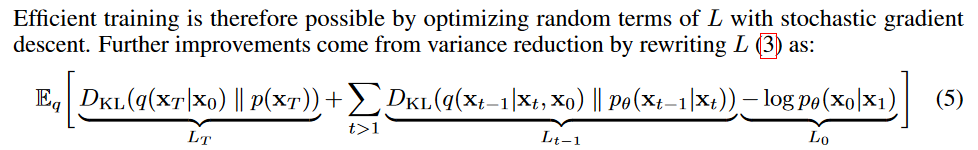
We see they decompose it into $L = L_0 + L_1 + … + L_T$ and that each $L_t$ term except for $L_0$ are a KL-divergence (or Kullback–Leibler (KL) divergence is a function that computes the difference or distance between two probability distributions) between $q$ and $p_\theta$ which are two Gaussian distributions. The loss can then be rewritten as an L2-loss by using the means of each distribution.

Finally, they do one final reparametrization on the mean that enables the network to predict the added noise on an image instead of predicting the mean itself. This means that the network actually becomes a noise predictor rather than a Gaussian mean predictor. The mean reparametrization looks like this:

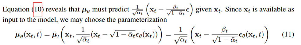
Plugging this into the Gaussian probability density function (PDF) leads us to the following loss function that computes the difference in mean :

$L_{t-1} = || \mathbf{\epsilon} - \mathbf{\epsilon}_\theta(x_t, t) ||^2 $

$L_{t-1} = || \mathbf{\epsilon} - \mathbf{\epsilon}_\theta( \sqrt{\bar{\alpha}_t} x_0 + \sqrt{(1- \bar{\alpha}_t) } \mathbf{\epsilon}, t) ||^2.$

If you want more more details on the calculations, see section 3.2 of the paper.

$x_0$ being the initial unmodified image, $\mathbf{\epsilon}$ is the noise level at time step $t$ and $\mathbf{\epsilon}_\theta (x_t, t)$ is our neural network.

After all this simplification we just end up with a simple Mean Squared Error (MSE) between the true noise $\mathbf{\epsilon}$ and the Gaussian noise predicted by our neural network $\mathbf{\epsilon}_\theta (x_t, t)$.

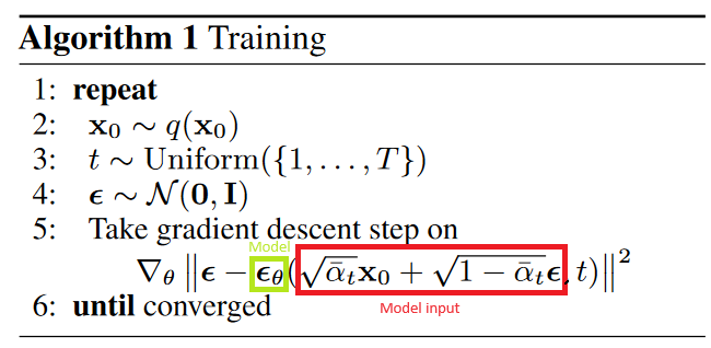
The final training procedure is:

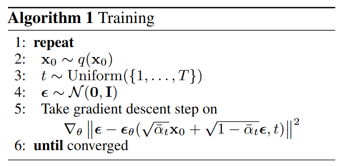
In other words:

• We take a random image $x_0$ from the train dataset $q(x_0)$
• We sample a noise level $t$ uniformally between $1$ and $T$, meaning we want it to be at a random time step
• We sample some noise from a Gaussian distribution and corrupt the input by this noise at level $t$
• The neural network is trained to predict this noise based on the corruped image $x_t$. It’ll try to find the noise that was applied on $x_0$ based on the fixed schedule $\beta_t$.

That was a lot of reparametrization but we got there, now let’s try to understand the procedure to generate an image.

Generating an Image by Sampling

Generating an image is actually quite simple (relatively to what we just saw). We say that we “sample” an image because we get it from a distribution. In our case, we did all this hard work to be able to work with Gaussian distributions, so let’s use it.

The process to sample an image is basically to start from a pure noise image, reverse the noise as much as we can until we end up with a clean image.

To sample from a standard Gaussian (or Normal) distribution we just do $\mathbf{z} \sim \mathcal{N}(\mathbf{0}, \mathbf{I})$ and since we want to sample from our own Gaussian distribution for which we learned the mean and variance parameters, let’s scale our samples: $\mathbf{z_{\theta, t}} = \mathbf{\mu_\theta(x_t, t)} + \sigma_t \mathbf{z}$, and $\mathbf{z_{\theta, t}}$ is our approximate to $x_{t-1}$ having started from $t=T$, we want to go to $t=0$ using repetitive sampling until we get $x_0$, a real image.

In our case: $x_{t-1} = \frac{1}{\sqrt(\alpha_t)}(x_t - \frac{\beta_t}{\sqrt{1 - \overline{\alpha_t}}} \epsilon(x_t, t) ) + \sigma_t z$, where $\mathbf{z} \sim \mathcal{N}(\mathbf{0}, \mathbf{I})$ from our simple Gaussian distribution.

We end up with the following algorithm for generating an image:

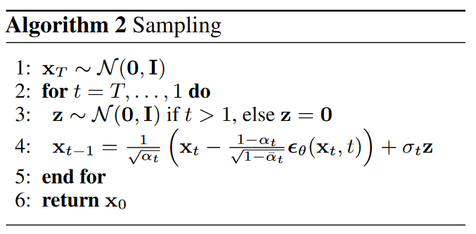
We finally have the full algorithm to start implementing our new model!

Something to Note

Diffusion Models also exist under different forms mathematically speaking that all have different names (like Score-based generative models, SDE-based generative models, Langevin dynamics, etc) that people discovered at different times. To learn more, read this.

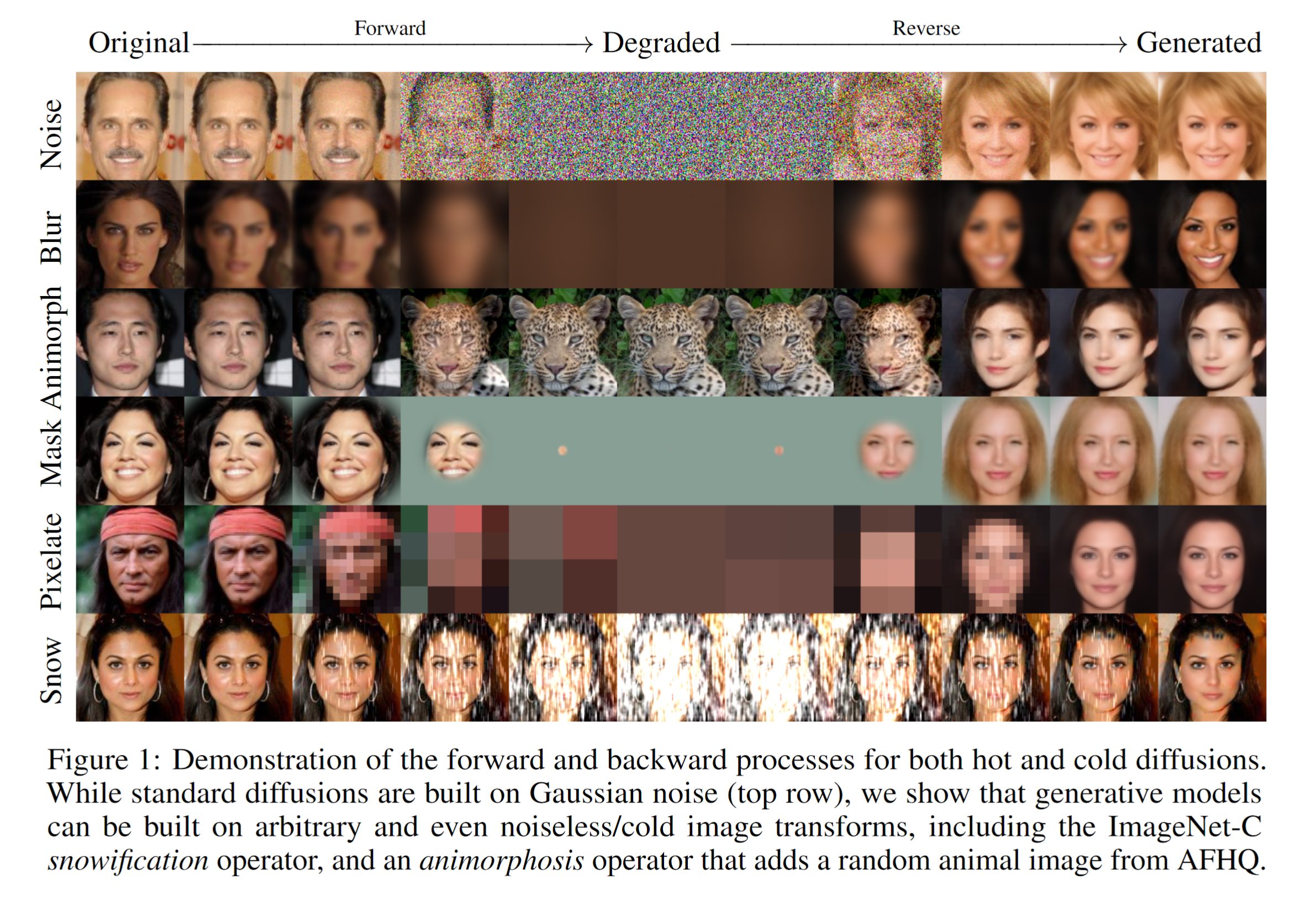
Also, some research (“Cold Diffusion: Inverting Arbitrary Image Transforms Without Noise”, Bansal et al. 2022) has been done to actually show that diffusion models don’t need to invert actual noise but can actually invert any arbitrary function like blur, masking, snowification (adding a snow like effect) or even animorphosis (transforming into an animal)!

Let’s Implement This!

Ok, we went quite deep in the theory, but we’re finally at the implementation phase. Let’s train a model to generate some images!

First, clone the repository found here and you’ll find many helper files in the practical_work_3_ddpm/ folder and you will be using the provided notebook in which you will complete functions by following the exercises.

Loading and Process the Dataset

Let’s generate images from the Fashion MNIST dataset. It’s basically the equivalent of the handwritten digit dataset MNIST but for clothes, so it’s a more complex dataset. There are 10 classes of clothes and the images are grayscale and $28x28$ in size to match the original MNIST dataset.

Let’s use 🤗 Datasets to load this dataset very easily:

from datasets import load_dataset

dataset = load_dataset("fashion_mnist") # load dataset from the hub
image_size = 28 # Height = Width = 28
channels = 1 # Grayscale image so 1 channel1
batch_size = 128 # Works well on Google Colab with 16GB VRAM but modify this to match your hardware

The paper specifically says that each pixel values are converted from the $[0, 255]$ range into $[-1,1]$. They also apply random horizontal flips to the image to augment the data and say it increases “quality slightly”, so we’ll do it too:

from torchvision import transforms
from torch.utils.data import DataLoader

# Define the image transformations using torchvision
transform = Compose([
            transforms.RandomHorizontalFlip(), # Horizontal flips augmentation
            transforms.ToTensor(), # Convert to PyTorch tensor
            transforms.Lambda(lambda t: (t * 2) - 1) # Convert to the [-1, 1] range
])

# Transform function
def transforms(examples):
   # Apply the transformation on each train image
   # "image" is the key that contains the image data in the Fashion MNIST dataset
   examples["pixel_values"] = [transform(image) for image in examples["image"]]

   # We remove it since we transformed the image above to what fits us and we don't need the original image anymore
   del examples["image"]

   return examples

# Apply the transforms
transformed_dataset = dataset.with_transform(transforms).remove_columns("label")

# Create the dataloader that will output batches of our transformed train data
dataloader = DataLoader(transformed_dataset["train"], batch_size=batch_size, shuffle=True)

Let’s Pre-Compute the $\alpha$ and $\beta$ Values

As we went through the formulas in the theory section, we talked a lot about $\alpha$, $\overline{\alpha}$ and $\beta$ values. Let’s compute them first since we’ll need them later.

We know that our $\beta$ variance values come from a scheduler, so let’s implement this scheduler first.

$\beta$-Variance Schedule

In the paper, they choose the scheduler to be a simple linear schedule, meaning we get uniformly spaced points from a line. They get values in the range $\beta_1 = 10^{-4}$ to $\beta_T = 0.02$ and let’s set the total number of time steps $T = 600$. The implementation is very simple actually:

# timesteps is T
def linear_beta_schedule(timesteps, beta_start = 0.0001, beta_end = 0.02):
    betas = torch.linspace(beta_start, beta_end, timesteps)

    return betas

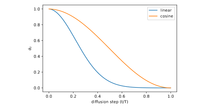
There’s a slight issue though, even if they choose the linear $\beta$ schedule , further research (Section 3.2 of “Improved Denoising Diffusion Probabilistic Models”, Nichol et al. 2021) shows that it is actually quite strong because noise grows very rapidly in the first half of the time steps and we even start having issues recognizing the original image with the naked eye. This means that a lot of the time steps almost become unusable for training the model since it will struggle a lot for a while with heavy noise.

The new proposed cosine schedule is defined as follows:

$\overline{\alpha_t} = \frac{f(t)}{f(0)}, f(t) = cos(\frac{t/T + s}{1 + s}.\frac{\pi}{2})^2$, with $s = 0.008$.

To go from this definition to variances $\beta_t$, we note that $\beta_t = 1 - \frac{\overline{\alpha_t}}{\overline{\alpha_{t-1}}}$. To help you with this part, notice that for $\overline{\alpha_{t-1}}$ you’ll take all the $\overline{\alpha_t}$ we computed above and remove the last element of the array. You’ll notice that both arrays don’t have the same shape anymore, so you’ll have two choices, either remove the one element from the $\overline{\alpha_t}$ so it matches the $\overline{\alpha_{t-1}}$ array or you will pad the $\overline{\alpha_{t-1}}$ array with one more element. Up to you to try and see what works best for you.

Finally, we’ll clip the final $\beta$ values to the range $[0.0001, 0.02]$ to prevent singularities at the end of the diffusion process near $t = T$. In the paper, they clip in the range $[0.0001, 0.999]$, but I find this to be too strong for the $\alpha_t$ which can create numerical instabilities and the network would require more dropout to handle this, so we’ll stick with the range $[0.0001, 0.02]$ similarly to the linear schedule range.

Remember that the cosine schedule should give you values that go towards $0.02$ less quickly, at the beginning and in the middle of the array, than the linear schedule. So compare your values between the two schedules. The last $\beta$ values matters less since it’s very close to full of noise anyway.

In the end, this new schedule should in theory converge to better images given enough timesteps and enough training time compared to the linear schedule. On this dataset the difference will be a bit harder to see, but in general it gives better results.

Read section 3.2 of “Improved Denoising Diffusion Probabilistic Models”, Nichol et al. 2021 carefully.

This is the function you’ll need to complete:

# timesteps is T
def cosine_beta_schedule(timesteps, s=0.008):
   """
   cosine schedule as proposed in https://arxiv.org/abs/2102.09672
   """
   steps = timesteps + 1
   t = torch.linspace(0, timesteps, steps)
   
   # COMPLETE THIS

   # Clip betas values
   return torch.clip(betas, 0.0001, 0.02)

Let’s Compute the Rest of The Constants

With the above we now have computed our $\beta_t$ values. We now needs the $\alpha_t$ values, and after we need the $\overline{\alpha_t}$. On top of that we’ll precompute some others values we’ve seen in several places in the previous sections like $\frac{1}{\sqrt{\alpha_t}}$, $\sqrt{\overline{\alpha_t}}$ and $\sqrt{1 - \overline{\alpha_t}}$. Finally, we’ll pre-compute our posterior variance $q(x_{t-1} | x_t,x_0)$ to use for the forward process.

1. $alphas = 1.0 - betas$
2. $alphas \_ cumprod = \prod_{t=0}^{T} alphas$
   • Look into torch.cumprod
3. $sqrt\_recip\_alphas = \sqrt{1.0 / alphas}$
4. $sqrt \_ alphas \_ cumprod = \sqrt{alphas \_ cumprod}$
5. $sqrt \_ one \_ minus \_ alphas \_ cumprod = \sqrt{1.0 - alphas \_ cumprod}$
6. $sigma = betas * (1. - alphas \_ cumprod \_ prev) / (1. - alphas \_ cumprod)$: $alphas \_ cumprod \_ prev$ is already computed for you below.

Complete the following code with the above formulas and add it to your notebook:

timesteps = 600

# define beta schedule
betas = linear_beta_schedule(timesteps=timesteps) # or `cosine_beta_schedule(timesteps=timesteps)`

# define alphas
alphas = ...
alphas_cumprod = ...

# This is just the previous step of the cumulative product above
# It's just alphas_cumprod without the last value and with a 1.0 padding at the beginning
alphas_cumprod_prev = F.pad(alphas_cumprod[:-1], (1, 0), value=1.0)

sqrt_recip_alphas = ...

# calculations for diffusion q(x_t | x_{t-1}) and others
sqrt_alphas_cumprod = ...
sqrt_one_minus_alphas_cumprod = ...

# calculations for posterior variance q(x_{t-1} | x_t, x_0)
sigma = ...

This will help us code the few formulas for diffusion process much more easily.

Let’s Implement The Inference

Take a look at the inference loop (or sampling as they call it in DDPM specifically):

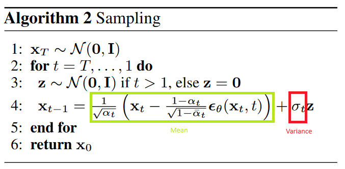
Let’s explain this line by line so you can implement it right after:

1. $x_t \sim \mathcal{N}(\mathbf{0}, \mathbf{I})$: Here we just sample a noisy image from a Gaussian distribution. This is already implemented for you in the p_sample_loop function this way: torch.randn(shape, device=device)
   • You’ll find this function in the notebook in the repository
2. $\mathbf{for}$ $t = T, … , 1$ $\mathbf{do}$: This is simply a for loop from the maximum time step $t = T = 600$ to $t=1$. The reverse diffusion process is going from the noisy image to an actual generated image, that’s why we reverse the loop. This loop is already implemented for you in the p_sample_loop function as: for i in tqdm(reversed(range(0, timesteps))):

You will be implementing line 3 and 4, and to help you we’re going to implement it using a function that will help us extract for a given time step $t$ the $\alpha_t$, $\beta_t$ from all the $alphas$ and $betas$ we computed above. Just use this function that’s already provided in your notebook:

# This function helps us extract from the array of, for example, all `betas`, the current time step `beta_t`, basically adds the `_t` part our formulas need.
def extract(a, t, x_shape):
    # Get the current batch size
    batch_size = t.shape[0]
    # Get all values from the last axis at the timestep t
    out = a.gather(-1, t.cpu())
    # Reshape the output to the correct dimensions
    return out.reshape(batch_size, *((1,) * (len(x_shape) - 1))).to(t.device)

Let’s dive into the details of line 3 and 4:

3. $\mathbf{z} \sim \mathcal{N}(\mathbf{0}, \mathbf{I})$ if $t > 1$, else $\mathbf{z} = 0$. Let’s do each branch of the condition:
   • $\mathbf{z} = 0$ if $t == 0$: This basically sets the right part of the addition on line 4 (red rectangle) $\sigma_t \mathbf{z}$ to $0$, so we just need to return the mean on the right.
   • $\mathbf{z} \sim \mathcal{N}(\mathbf{0}, \mathbf{I})$ if $t > 1$: In this part, we just sample noise that has the same shape as $x_t$.
     • Look into torch.randn_like
4. This formula just lets us get nearer to a generated image, one step at a time. Let’s separate it into two parts, the mean (green highlighted rectangle) and the variance (red highlighted rectangle). Remember that this line is simply $x_{t-1} = \mu_t + \sigma_t \mathbf{z}$, so we just scale our Gaussian noise with the mean $\mu_t$ and variance $\sigma_t$:
   • The mean $\mu_t = \frac{1}{\sqrt{\alpha_t}} (x_t - \frac{1 - \alpha_t}{\sqrt{1 - \overline{\alpha_t}}} \mathbf{\epsilon_\theta}(x_t, t))$. We already precomputed some of the values in the previous section already. Let’s decompose it again:
     • $sqrt \_ recip \_ alphas \_ t = \frac{1}{\sqrt{\alpha_t}}$: and let’s not forget to apply extract(...) so we get $sqrt \_ recip \_ alphas \_ t$ for this specific time step $t$ from all the $sqrt \_ recip \_ alphas$ we already precomputed above. Applying it is simple and you’ll do the same for every other $* \_ t$ variables, so here’s to do it for this step as an example: sqrt_recip_alphas_t = extract(sqrt_recip_alphas, ts, x_t.shape)
     • $betas \_ t = 1 - \alpha_t$: We also need to apply extract(betas, ts, x_t.shape) from our precomputed $betas$ to get $betas \_ t$.
     • $sqrt \_ one \_ minus \_ alphas \_ cumprod \_ t = \sqrt{1 - \overline{\alpha_t}}$: We already precomputed all the $sqrt \_ one \_ minus \_ alphas \_ cumprod$ in our constants, so you can just sample it with extract(...) like above.
     • $\mathbf{\epsilon_\theta}(x_t, t)$ is just applying our model, so it’s equivalent to simply calling model(x_t, ts).
   • We already precomputed posterior variance $\sigma$, which we’ve already computed thanks to the $betas$ and $alphas$, so we just need to apply extract(...) to it to get $\sigma_t$ and that’s it for this part.

Now, just assemble all the formulas above to get the final formula from Algorithm 2: Sampling.

# torch.no_grad just tells PyTorch not to store any gradients for this because we don't need them and it takes a lot of memory if it stores them
@torch.no_grad()
def p_sample(model, x_t, ts, current_t):
   """
      model: Our model we'll create later
      x_t: The noisy image of current time_step `t`
      ts: All the $t$ for the current time step, basically an array with only `t` times the batch size. Remember that we are always computing our formulas for multiple images at the same time (aka all imaages in the batch).
      current_t: The $t$ integer value from the `ts` array. It's more convenient to have by itself if we want to do the if condition we saw. You could also take the first (or any other) value from the `ts` array, but less convenient.
   """

   # Extract the current time step constants `*_t` here

   # COMPLETE THIS
   sqrt_recip_alphas_t = ...
   betas_t = ...
   sqrt_one_minus_alphas_cumprod_t = ...

   mean_t = ...

   # The condition line 3 in the algorithm
   if current_t == 0:
      # `if t = 0: z = 0` so we can just return the `mean_t`
      return mean_t
   else:
      # COMPLETE THIS PART

      # sigma_t is the posterio variance
      sigma_t = ...
      # z is the noise
      z = ...

      return mean_t + ...

Let’s Implement The Training Loss

Take a look at the training loop again:

So, for example, if we want to extract $sqrt \_ alphas \_ cumprod \_ t$ from $sqrt \_ alphas \_ cumprod$, we simply do extract(sqrt_alphas_cumprod, t, x_0.shape), where sqrt_alphas_cumprod is one of the constants we computed above for simplicity, x_0 is the image we start from and t the current time step.

# forward diffusion
def q_sample(x_0, ts, noise=None):
   """
      x_0: The original image that we want to add noise to given the specific beta schedule we precomputed above
      ts: All the $t$ for the current time step, basically an array with only `t` times the batch size. Remember that we are always computing our formulas for multiple images at the same time (aka all imaages in the batch).
   """

   if noise is None:
      noise = torch.randn_like(x_0)

   # COMPLETE THIS
   sqrt_alphas_cumprod_t = extract(sqrt_alphas_cumprod, ts, x_0.shape)
   sqrt_one_minus_alphas_cumprod_t = extract(
      sqrt_one_minus_alphas_cumprod, ts, x_0.shape
   )

   # The red rectangle part in our formula
   model_input = ...

   return model_input

This is the complete loss function in which your function will get plugged:

# This function is already made for you, it computes the full loss from the training loop above using your implementation of `q_sample` (the red rectangle part)
# You can choose between 3 loss types, "l1", "l2" (or Mean Squared Error (MSE), like in the paper) or "huber" (or smooth l1) loss.
def p_losses(denoise_model, x_0, t, noise=None, loss_type="l1"):
   # The noise `epsilon` in our equation to which we compare our model noise prediction
   if noise is None:
      noise = torch.randn_like(x_0)

   # This is where `q_sample` is being used
   # `x_noisy` is basically our model input
   x_noisy = q_sample(x_0=x_0, t=t, noise=noise)

   # epsilon_theta from our formula in the green rectangle
   predicted_noise = denoise_model(x_noisy, t)

   # The `|| epsilon - epsilon_theta ||^2` part of the equation
   # The derivative part is only computed later in the training loop by PyTorch as we've been doing for all our models up until now
   # You can choose between 3 losses, L2/MSE loss is the one from the paper
   if loss_type == 'l1':
      # Same as L1 without the power of 2
      loss = F.l1_loss(noise, predicted_noise)
   elif loss_type == 'l2':
      # The loss in the paper
      loss = F.mse_loss(noise, predicted_noise)
   elif loss_type == "huber":
      # The Huber loss might be slightly better in this case
      loss = F.smooth_l1_loss(noise, predicted_noise)
   else:
      # If we input any another loss
      raise NotImplementedError()

   # Return the final loss value
   return loss

The Model Architecture

Wait, we haven’t talked about the model architecture at all, have we?

To understand the neural network required for this task, let’s break it down step-by-step. The network needs to process a noisy image at a given time step and return the predicted noise in the image. This predicted noise is a tensor with the same dimensions as the input image, meaning the network’s input and output tensors have identical shapes. So, what kind of neural network is suited for this?

Usually, a network architecture called an Autoencoder is used here. Autoencoders feature a “bottleneck” layer (literally like the neck of a bottle where water comes out of at a lower specific rate) between the encoder and decoder. The encoder compresses the image into a smaller hidden representation, and the decoder reconstructs the image from this representation. This design ensures that the network captures only the most crucial information in the bottleneck layer.

In terms of architecture, the authors of the DDPM paper opted for an architecture that follows the backbone of PixelCNN++, which is a U-Net introduced by Ronneberger et al., 2015 (but based on a Wide ResNet). This architecture achieved state-of-the-art results in medical image segmentation at the time. Being an Autoencoder, a U-Net has a bottleneck that helps the network learn essential features. Additionally, it includes residual connections between the encoder and decoder, inspired by He et al., 2015’s ResNet, to improve gradient flow.

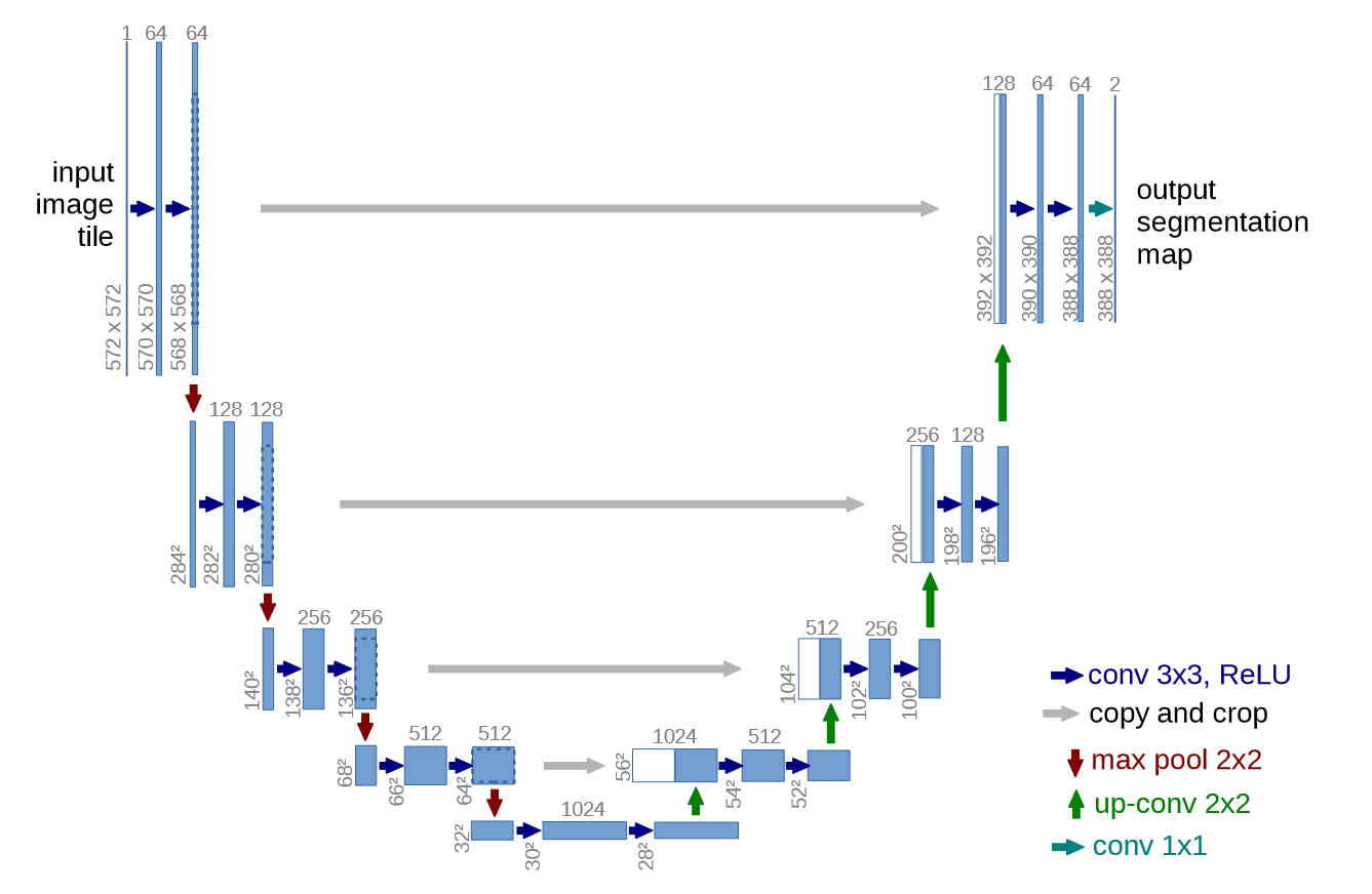
As shown in the figure, a U-Net model first downsamples the input image (reducing its spatial resolution) and then upsamples it back to the original size.

Let’s Look at our U-Net in More Details

Remember that our model $\epsilon_\theta(x_t, t)$ should predict, for each image in a batch and the current time step $t$, the noise that was added to each image, so we can remove it later.

Let’s look at the model’s inputs and outputs:

• Inputs:
  1. A batch of noisy images of shape $(batch \_ size, channels, height, width)$
  2. A batch of time steps $t$ of shape $(batch \_ size, 1)$
• Outputs:
  1. The noise added to each image at a specific time step $t$ of shape $(batch \_ size, channels, height, width)$

Our model is be made of several components:

• Positional Embeddings: To give our model a sense of time. It is based on the Transformers paper, “Attention Is All You Need” by Vaswani et al., 2017
• ResNet blocks: The Convolutional building blocks of this U-Net (Made of Conv2d -> Group Normalization -> SiLU Activation)
• Attention Module: This allows the neural network to focus its attention on the important part of the input. It is also based on the Transformers paper, “Attention Is All You Need” by Vaswani et al., 2017
• Group Normalization: A way to apply normalization, like Batch Normalization (BN). Group Normalization (GN) divides the channels into groups and computes within each group the mean and variance for normalization. The authors use this instead of Weight Normalization to simplify the implementation.

This is how they are assembled to form the final architecture of the U-Net:

1. A 2D Convolutional layer of kernel_size = 7 is applied on the input batch of noisy images. On top of that, we use the current input time step $t$ to compute our Positional Embeddings
2. In the downsampling stage (the left part going downward of the U-Net): We apply ResNet blocks with attention and residual connections (also called skip connections) followed by downsampling. This happens several time until we downsample enough to reach the bottleneck stage.
3. At the bottom middle part of the network, we have the bottleneck: ResNet blocks and attention are applied there
4. In the upsampling stage (the right part going upward of the U-Net): We apply ResNet blocks with attention and residual connections (also called skip connections) followed by upsampling. This happens several time until we upsample enough to reach the the output stage.
   • This stage receives skip connections from layers at the same height in the downsampling stage: This helps the model reuse previous information it might have lost in the bottleneck and also helps a lot with gradient flow (Vanishing gradients problem).
5. Finally, a ResNet block is applied followed by a final convolution to get the correct dimensions for output

Let’s Implement the U-Net’s ResNet Block

We will complete the following function to implement our ResNet block:

class Block(nn.Module):
    def __init__(self, dim, dim_out, groups = 8):
        super().__init__()
        
        # COMPLETE THIS

    def forward(self, x):

        # COMPLETE THIS

You should complete this function in this Python file.

We said previously that our U-Net has ResNet blocks, and these blocks are made of:

1. 2D Convolution: Conv2d(dim, dim_out) with a kernel size of $3$ and a padding of $1$.
2. Group Normalization: With the number of groups to separate the channels into being groups and the number of channels expected in the input being dim_out.
3. SiLU (or Swish) Activation: It is simply a scaled logistic sigmoid you can directly apply at the end. SiLU/Swish being unbounded above, bounded below, non-monotonic, and smooth are all advantageous during training for gradient flow, it’s also an easy replacement for ReLU. Read the Swish paper for more details.

They are applied one after the other in this order: Conv2D -> GroupNorm -> SiLU.

So, How Do We Teach The Concept of Time to Our Model?

As we’ve seen, the diffusion process is time dependent where we have the value $t$ to help us keep track of time. Each time step $t$ works at a specific noise level, so to help our model operate at these specific noise levels, we’ll need to feed it the $t$ value.

To implement this, the authors actually use the positional encoding method from Transformers (From the foundational paper “Attention Is All You Need” by Vaswani et al. 2017).

They introduced Sinusoidal Positional Embeddings that use $sin(x)$ and $cos(x)$ functions that are cyclic functions that don’t need to be learned! How can we encode positioning (in this case, time, which is a form of positioning on the axis of time $t$) using these two functions?

The Transformer paper proposes the following functions to generate specific frequencies at each position $pos$ (or timestep $t$ for us): (Section 3.5, Positional Encoding)

$PE_{(pos, 2i)} = \sin \left( \frac{pos}{10000^{\frac{2i}{d}}} \right)$

$PE_{(pos, 2i+1)} = \cos \left( \frac{pos}{10000^{\frac{2i}{d}}} \right)$

They basically create several sine and cosine functions with different frequencies, so imagine creating a matrix where each row will contain a new sine/cosine function that oscillates different (higher or lower frequency for each). This basically helps introduces assign a frequency to each time step, meaning that at a specific time step we will add a specific frequency to its embeddings so that, the exact same input at a different time step will have this specific frequency added that will say to the network “Ok, it’s the same image but with a different time step, so it should be processed differently according to the current noise level of timestep $t$”.

Let’s Implement Sinusoidal Positional Embeddings

In our specific case, each input will have only one type of sine/cosine frequency for the entire image since the model only sees one image per timestep $t$ in the input. So we can only output one specific sine/cosine frequency for a given timestep $t$. So let’s rewrite the formulas for our case to only generate one frequency at a timestep $t$:

1. We want sine and cosine to each contribute half to the frequency function, so we’ll need to define a half_dim variable that will just be: half_dim = image_dim / 2

2. For the term $10000^{\frac{2i}{d}}$, we will use logarithms for computational stability (to reduce the range of numbers so we don’t overflow) and simplicity, we can rewrite it as $log(10000^{\frac{2i}{d}}) = \frac{2i}{d}log(10000)$. In the code we can simplify this to: $embeddings = log(10000)/(half \_ dim - 1)$

3. Now, let’s generate the values we need to add to our frequency: We need to generate a range of numbers $[0, 1, 2, …, \frac{d}{2} - 1]$ which we will multiply by $-embeddings$ from above to scale them logarithmically, so now we have: $embeddings = exp(- \frac{log(10000)}{half_dim - 1})$.

   • Quick explanation: Mathematically, using $exp(x)$ rules, we have $freq(i) = 10000^{- \frac{2i}{d}} = exp(- \frac{2i}{d} log(10000))$ that matches what the Transformers paper says

4. Let’s scale the current position (or time step $t$) by doing an outer product with our embeddings: $embeddings = time_step * embeddings$, where $time_step$ is basically the time step $t$ we’ve been talking about this entire time

   • Hint: Make sure to apply it on the correct PyTorch tensor dimensions. You might need to extend the axis size if needed. Look at each tensor’s shape (embeddings should be a row vector and time should be a column vector at the end) while trying to implement this part

5. Finally, we need to concatenate the sine and cosine embeddings along the last dimension: $concatenate(sin(embeddings), cos(embeddings))$

Here’s the code boilerplate you’ll need to complete, you’ll find it here in the Github repo:

class SinusoidalPositionEmbeddings(nn.Module):
    def __init__(self, dim):
        super().__init__()
        self.dim = dim

    def forward(self, time):
        device = time.device # The device on which to put the tensors we create below

        half_dim = self.dim // 2 # Step 1
        embeddings = math.log(10000) / (half_dim - 1) # Step 2
        
        # COMPLETE THIS FOR THE REST OF THE STEPS 3, 4, 5
        
        return embeddings

Training The Model

In the notebook, we can now run the training loop with our implementation ready. We’ll see that it can take 10-50 epochs to converge to a useful result.

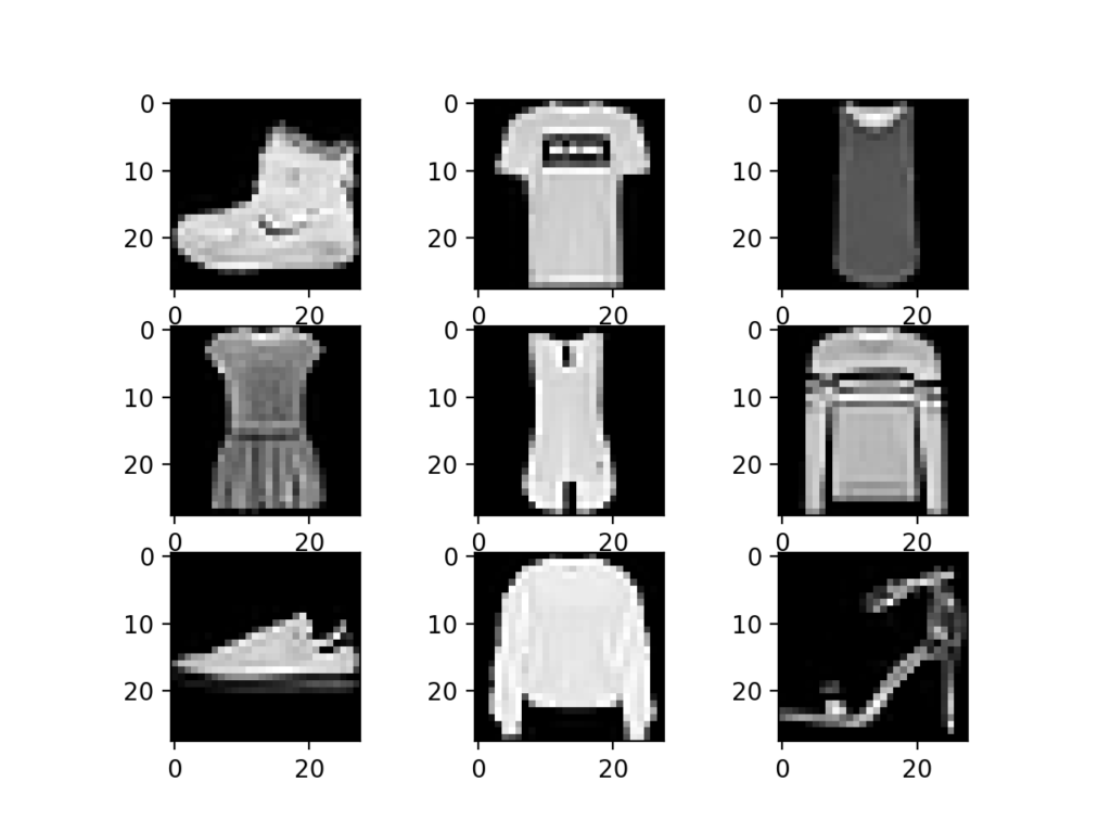
Running the training loop will get you to a result that looks like this after denoising:

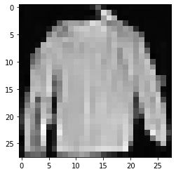
The results look simple since we haven’t trained the model for a long time, but this method can be scaled for more epochs, also on bigger datasets to produce better results but we need better hardware and longer training times.

You can also run inference at the end of the notebook yourself in the Test The Model section at the end, that will generate random images of clothes.

Bonus Exercises

ConvNext Architecture

You might have noticed that when we instantiated our Unet(...) model, we set use_convnext=False and resnet_block_groups=1. The code implements another architecture instead of ResNet, which is called ConvNext from the paper “A ConvNet for the 2020s”, Liu et al, 2022. This architecture tries to modernize ConvNets since recently, Vision Transformers (ViTs) have taken over ConvNets. The ConvNext paper argues that ViTs work well but it’s not only because of the Transformer architecture but also all the small architecture changes that we done on the side, so applying them to ConvNets should also help them reach the same performance, and it actually worked.

We trained our model on a simple dataset, now try training it on more complex datasets, that can have colored images or higher resolution. Keep in mind that this means you’ll need a better machine or much longer training time.

Here’s a list of simple datasets:

• CIFAR10: Contains 10 classes of some small random images (trucks, cats, etc)

• CelebA: Contains celebrity faces

• LSUN: LSUN has many variants, like LSUN Bedrooms with images of bedrooms, LSUN Church with images of churches, don’t ask me why, but they are good already made datasets to try.

These datasets are more complex and will require you have a better GPU or that you run it for longer.

You’re Done!

Great job, you made it this far!

Class Students

Send it on the associated MS Teams Assignment.

Anyone else

Send it to my email adress with the subject Practical Work 3: chady1.dimachkie@epita.fr

Don’t hesitate if you have any questions!

→ Coming Next: Practical Work 4