1. Build a Neural Network in PyTorch

May 17, 2024

In this first practical work, we’ll be experimenting with simple neural networks on simple datasets.

First, Get Setup

It’s recommended to use a Jupyter notebook since you’ll be doing some visualization.

Locally

You should have Jupyter installed and the following dependencies. You can use pip or any other dependency manager:

pip install torch matplotlib scikit-learn

You can add more dependencies if you think it is relevant.

In The Cloud (Google Colab)

Simply click here to open a Colab notebook in your browser. You’ll need to sign-in with you Google account.

In the first cell, add the following to install the dependencies:

!pip install torch matplotlib scikit-learn

Same here, you can add more dependencies if you think it is relevant.

Let’s Get Started

In this first practical work you’ll be creating a simple neural network in PyTorch to fit multiple simple datasets.

Let’s get started !

Why PyTorch?

PyTorch is one of the leading open-source machine learning frameworks to design, train and run inference on neural networks. It is developped by Meta AI.

A lot of machine learning software made by big tech companies is made using PyTorch, even Tesla for their Autopilot.

Our First Neural Network!

Let’s start with a linear function

Before starting and creating a neural network, we need to choose a dataset to use so we can experiment on.

To understand the basics when building a neural network, we’ll first create our own dummy dataset consisting of a simple linear looking function.

What’s a simple linear looking function you ask?

Something of the form $y = ax + b$, let’s say for example $y = -x + 5$, where $y$ will be our dataset that contains all the possible points that will be created by all the possible $x$ values we input.

Let’s recreate this function in PyTorch:

def create_dataset(n_data:int = 100, a:float = -1.0, b:float = 5, scale:int = 15) -> torch.tensor:
    # Generate random data as inputs
    x = torch.rand(n_data, 1) * scale  # n_data=100 random numbers scaled between 0 and scale

    # Calculate corresponding y values
    y = a * x + b

    # We center the data by using the mean of all values
    return x - torch.mean(x), y - torch.mean(y)

Now, let’s make it slightly more interesting and make it only look like it’s a linear function. For that we’ll add some noise. You’ll see later that the data you find in real world scenarios has a lot of noise, meaning it’s usually not perfect.

def create_dataset(n_data:int = 100, a:float = -1.0, b:float = 5, scale:int = 15) -> torch.tensor:
    # Generate random data as inputs
    x = torch.rand(n_data, 1) * scale  # n_data=100 random numbers scaled between 0 and scale

    # Calculate corresponding y values
    y = a * x + b

    # Add some noise
    noise = torch.randn(y.shape) * 2  # Gaussian noise with standard deviation of 2
    y = y + noise

    # We center the data by using the mean of all values
    return x - torch.mean(x), y - torch.mean(y)

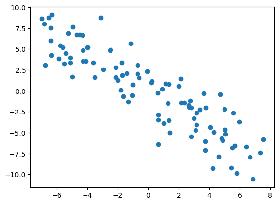
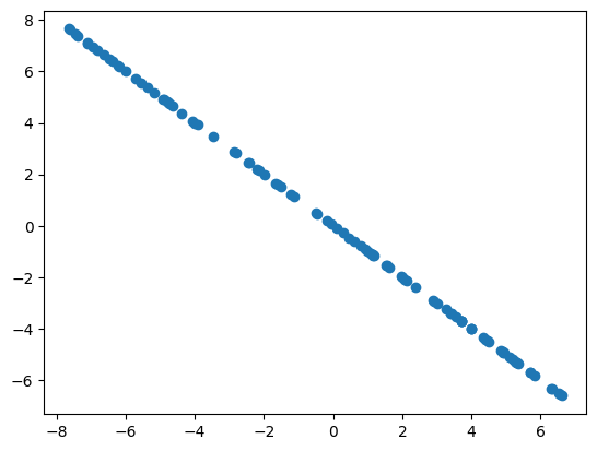
The data looks linear if you look at it from far away which is what we wanted. Let’s try to make a simple neural network that will learn to approximately recreate this function.

Creating a Linear Neural Network

Let’s first start by describing what a linear neural network looks like:

$y = W^ta + b_w$ where $W$ is the weights matrix and $b$ is the bias. Unsurprisingly, it reminds us of the above previous linear equation $y = ax + b$.

From this equation, we can see that if we’re able to learn a $W$ that is close to $a$ and a $b_w$ close to $b$ then we’ll have approximated our function.

class Net(torch.nn.Module):
    """
    A simple 1 layer neural network with no activations
    """

    def __init__(self, n_feature:int, n_output:int):
        super(Net, self).__init__()
        
        # Create a linear layer
        self.hidden = torch.nn.Linear(n_feature, n_output)

    def forward(self, x:torch.tensor):
        # Use the linear layer
        x = self.hidden(x)

        return x

The above class is very simple, it simply creates one linear layer that will be our entire neural network. You’ll see that this Linear layer is the basis of most neural networks, even the most complex ones.

We have two functions, the __init__ function just initializes the network. Basically, we want our $W$ and $b_w$ values to have an initial value and PyTorch automatically initializes our variables in a way that will make the network converge quickly. You can read more about initialization here, but we’ll come back to it later.

Let’s instanciate the neural network:

# We define the network
net = Net(n_feature=1, n_output=1)

As simple as that!

The network only takes one input and outputs a single number since we want the network to map each $x$ to its corresponding $y$ value by doing the $ax + b$ transformation.

Training the network

The Theory

Training a neural network means that we want to find a path towards one of the best solutions to our problem. The solution should be the best set of weights we can find (when our model converges and has the desired accuracy) from our starting point (the initialization of the network). How do we go from a starting point to a solution, we need to use an algorithm that helps us navigate there.

One of these algorithms is called gradient descent: gradient because we use derivatives and descent because we use these derivaties to guide us towards a good solution in the loss landscape.

What’s the loss function?

The loss function is a function that helps us compute a distance between of how far or close are our model’s prediction compared to what it’s supposed to answer (the ground truth). The loss function needs to be differentiable everywhere.

A simple and common loss function is the Mean Squared Error loss (also called squared L2 norm): $\frac{1}{n}\sum{(y_i - \hat{y}_i)^2}$, where $y_i$ is the ground truth and $\hat{y}_i$ is the predicted value from our model.

There are many more loss functions and we’ll see a few others along the way.

Ok, so what’s the loss landscape?

Take a look at this mountain looking picture:

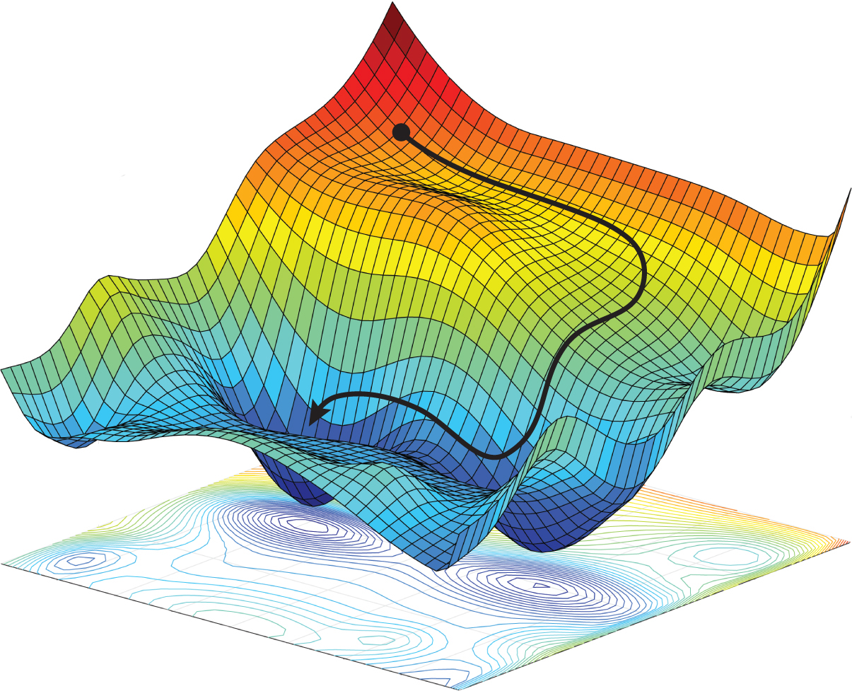
This is basically a representation of the loss values around the weight space of the network: What this means is that for each possible weights our networks can have (it’s a very large number so we usually only ever explore a few like what you see on the image), we can plot how it performs thanks to the loss function.

The lower we are in the landscape, the closer we get to a good solution. Furthermore, you can see that we start from a point quite high in the lanscape (the pseudo-random initialization of the network which we hope is good enough) and then, using an optimizer, we explore by following the gradients of what the loss is telling us until we reach a good enough weight set where our model performs well.

How do we navigate this landscape?

To navigate this landscape we’ll use what’s called an optimizer. The optimizer will follow what the derivates of the loss function at a specific time step $t$ is telling us and will take the best guess as to where to go given this information.

Most neural network optimizers are based on Gradient Descent (GD). This algorithm looks like this:

$W_{i+1} = W_i - lr * D_{loss}(W_i, X_{train}, y_{train})$, where $W_i$ are the current weights of the model, $D_{loss}$ is the loss function’s derivative that takes as input the current model weights $W_i$ to compute predictions on the training set $X_{train}$ and compare the model output (which we called $\hat{y}$ earlier) to the ground truth labels $y$.

We iterate on this until we find a model that performs well on our test data, which should be correlated to a low loss value.

In Practice

In practice, PyTorch does everything for you and defines preexisting algorithms we can reuse.

Above we said that we needed two things:

• An algorithm to find the best path to a good set of weights: This is called an optimizer and PyTorch offers a lot of different ones in torch.optim.
• A loss function to define how well our model is performing at each time step: torch.nn.*Loss offers a lot of loss functions.

In our case, we’ll use:

• Optimizer: Stochastic Gradient Descent (SGD)
• Loss function: Mean Squared Error (MSE)

In terms of code, it’s quite simple to create these two objects:

# Instantiate an SGD Optimizer that will work on our network's parameters (weights) with a learning rate of 0.005
optimizer = torch.optim.SGD(net.parameters(), lr=0.005)

# Instantiate the MSE Loss
loss_func = torch.nn.MSELoss()

And then to apply gradient descent and compute the loss function, we simply do:

# We simply call the function we made in the previous chapter
# It'll generate our linear looking dataset
x, y = create_dataset()

for t in range(num_steps):
    # Compute predictions from our training set `X_train`
    prediction = net(x)

    # The inputs to the loss function are:
    # 1. Our model's current predictions
    # 2. the target outputs y_train
    loss = loss_func(prediction, y)     

    # We need to clear the gradients from the previous iteration
    # because PyTorch stores them in case we need them.
    # In our case we don't need to remember what happened the previous step
    optimizer.zero_grad()
    # We compute backpropagation to get the gradients
    loss.backward()
    # We do one iteration of SGD
    optimizer.step()

And that’s it!

No formulas are needed on our end, PyTorch computes everything internally.

Let’s look into what’s happening

Let’s plot our dataset and the trained model’s predictions as it learns to predict the train data:

As we can see, our model converges very fast which makes sense since it really doesn’t have much parameters to learn to represent our dataset. On top of that, our network isn’t very expressive in what it can do, it can basically only fit a line so that’s why every point is actually on a line. It can’t fit the intricacies of our dataset. We also plot the loss function’s value which keeps decreasing the better we are able to fit the train data.

Let’s make the data more complex

Now, this model is basically useless since it can only fit a linear shape. Let’s see what happens when we ask this same model to fit a more complex non-linear dataset.

Let’s make a dataset from the pow function with some added noise as usual:

def create_dataset(n_data:int = 100, a:float = 2, b:float=0.2) -> torch.tensor:
    # We create n_data evenly spaces points from -1 to 1
    # x from -1 to 1 to get the full curvy shape of the power function
    x = torch.unsqueeze(torch.linspace(-1, 1, n_data), dim=1)

    # Pow function with added noise
    y = x.pow(a) + b * torch.rand(x.size())

    # Center the data
    return x - torch.mean(x), y - torch.mean(y)

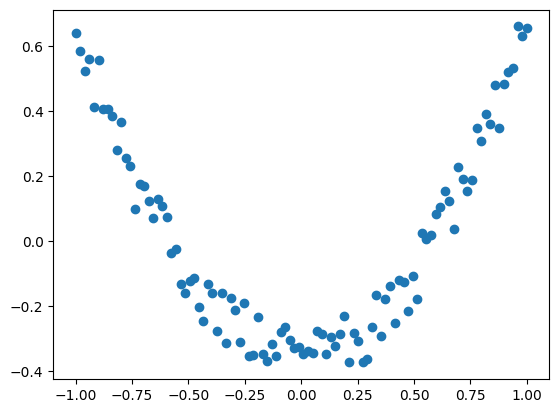
Let’s fit the same model on this dataset:

The model is trying its best to use a line to describe a more complex shape, but it clearly doesn’t work. It’s like explaining to someone living in a 2D world what a 3D world looks like, it’s not simple.

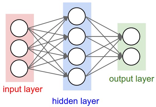
Creating a Multi-Layer Non-Linear Neural Network

Let’s move onto a more complex (but not so complex) model to fix this!

We’re going to do some slight changes to our previous model

class Net(torch.nn.Module):
    def __init__(self, n_feature, n_hidden, n_output):
        super(Net, self).__init__()
        # We add a hidden layer
        self.hidden = torch.nn.Linear(n_feature, n_hidden)
        # output layer
        self.predict = torch.nn.Linear(n_hidden, n_output)

    def forward(self, x):
        # We add a non-linear activation function at the output of our new hidden layer
        x = F.relu(self.hidden(x))
        x = self.predict(x)
        return x

net = Net(n_feature=1, n_hidden=10, n_output=1)

Let’s run it with the same code as previously on the new dataset with a slightly different learning rate of lr=0.5.

It fits our more complex dataset much better!

Teaching Another Task to Our Neural Network: Classification

We’ve been doing regression so far, meaning we’ve only been trying to match a dataset’s shape. Let’s now move onto classification which is a way to separate different categories within a dataset.

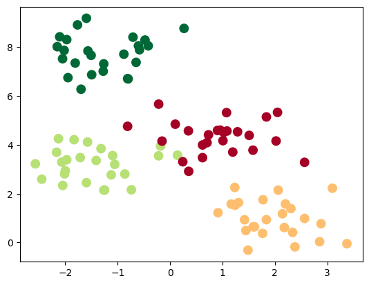
For that, let’s make yet another dataset:

from sklearn.datasets import make_blobs

def create_dataset(n_samples = 200, n_features = 2, n_classes = 2, cluster_std=0.7):
    X, y = make_blobs(n_samples=n_samples, cluster_std=cluster_std, centers=n_classes, n_features=n_features, random_state=0)
    
    return torch.from_numpy(X).float(), torch.from_numpy(y).long()

This time we’re using make_blobs from scikit-learn that enables us to generate what they call “blobs”, which are just several groups (or clusters) of data points. Let’s display it:

n_samples = 100
n_features = 2
n_classes = 4

x, y = create_dataset(n_samples=n_samples, n_features=n_features, n_classes=n_classes)

plt.scatter(x.numpy()[:, 0], x.numpy()[:, 1], c=y.numpy(), s=100, lw=0, cmap='RdYlGn')
plt.show()

Let’s reuse the exact same neural network architecture as earlier and only the number of features and the numbers of outputs:

net = Net(n_feature=n_features, n_hidden=10, n_output=n_classes)

We’ll also change the loss function since we are now doing classification instead of regression:

loss_func = torch.nn.CrossEntropyLoss()

This is what the Cross-Entropy loss looks like: $-\sum_{i=0}^Ly_i\log(p_i)$ where $p_i$ is the prediction from our model and $y_i$ is respective ground truth label.

In the case of 2 classes only, the loss can be simplified to this: $-{(y\log(p) + (1 - y)\log(1 - p))}$

If you want more details on Cross-Entropy, you can read more here.

Ok, now let’s run the training with the above changes:

Bonus

Bring Your Own Dataset!

We’ve only been working on simple datasets so far, let’s make it more interesting and work on something more useful.

Please pick one of the following datasets to work on:

• Iris plants dataset (Classification)
• Diabetes dataset (Regression)
• Linnerrud dataset (Regression)
• Wine recognition dataset (Classification)
• Breast cancer wisconsin (diagnostic) dataset (Classification)
• Optical recognition of handwritten digits dataset (Classification)

Each one of these datasets is easily downloadable using scikit-learn. You’ll find the loading functions here.

Tips to Get Started

Study the Dataset

Do a quick EDA (Exploratory Data Analysis) on your dataset. This is critical to understand the structure, contents, and relationships within the data:

• Look at the shape (rows, columns, etc) of your dataset
• Look at the data manually first to get a feel of what it looks like and what kind of data it is
• Generate a few statistics on the dataset, like mean, median, range, etc for each column

There are many other steps you can add, but here let’s keep it simple, we just want to understand how much input features are needed and how many outputs the model will have and what the data looks like in general.

Normalize The Values

Apply simple normalization to your dataset like centering values around $0$ (substracting the mean of the data to each value) and scaling the standard deviation to $1$ (dividing each value by the standard deviation).

Using scikit-learn you can do it very simply using StandardScaler for example.

Split into a Train/Test Set

If you dataset doesn’t already provide a test/validation set, you’ll have to do it manually. This is standard practice since you want to make sure you evaluate your model on data it hasn’t seen before to see if it generalized correctly from the train set you gave it. Ideally, if you have enough data, making a validation set is also a good practice, since it helps you test on some data the model hasn’t seen to track performance progress during training.

Using scikit-learn again you can do it very simply using the train_test_split function.

Accuracy Metrics

Make sure your metrics are adapted to your task.

For Classification

For classification tasks, look into metrics such as F1 Score, precision, recall, accuracy. You can even plot a confusion matrix. All these metrics can be found in scikit-learn.

Also, you can look at the loss value for both train and test data.

Regression

For regression tasks, look into metrics such as Mean Absolute Error (MAE), Mean Squared Error (MSE), Root Mean Squared Error (RMSE) and R-squared (R²) Score. Again, they can all be found in scikit-learn.

Refine Your Model

If your model doesn’t perform well, it might be due to:

• Not having pre-processed the data correctly (normalization, cleaning values, etc)
• Not having the right architecture for the problem, maybe you have a lot of data and you need a bigger model (more layers or bigger hidden layers)
• Your learning rate and your optimizer that aren’t correctly set

Bonus

You’re Done!

Great job, you made it this far!

Class Students

Send it on the associated MS Teams Assignment.

Anyone else

Send it my email adress with the subject Practical Work 1: chady1.dimachkie@epita.fr

Don’t hesitate if you have any questions!

→ Coming Next: Practical Work 2